Utility Function - Exponential Utility Function

What is the Exponential Utility Function?

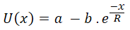
In economics and finance, the exponential utility is one specific shape of the Utility Function. People use it to turn real money into a sense of value. In plain terms, it captures how much a given gain or loss actually feels worth to you. A $1000 win does not feel twice as good as a $500 win to most people, and this curve is one way to show that. Written out, the exponential utility looks like this:

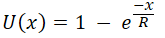
First form of the exponential utility function equation: U(x) equals 1 minus e to the power of negative x over R, where R is the risk tolerance.

You will also see it written this second way. The two forms say the same thing, just rearranged:

or

Generalized exponential utility function U(x) equals a minus b times e to the power of negative x over R, the form with scaling parameters a and b.

Here R is your Risk Tolerance, x is the real-world amount of money, and u(x) is the utility, the value of that outcome to you, measured in utils. The letters "a" and "b" are scaling numbers. The Decision Tree Software works these out for you from the smallest and largest amounts that are possible in your decision, which it asks you for.

Put the money gain on the X axis and your satisfaction on the Y axis, scored from 0 to 1, where 0 means no satisfaction and 1 means as happy as you can be. The exponential utility curve then looks like this:

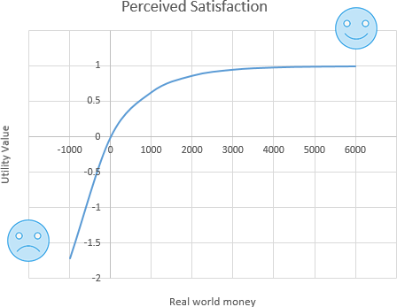
Plot of an exponential utility function curve showing concave shape that models risk-averse behavior, with the risk tolerance parameter R controlling concavity.

This curve is concave, which is what makes it good for showing risk aversion. The Risk Tolerance R sets how curved it is, and that curve is exactly what tells you how risk-averse the decision-maker is. The chart above uses a Risk Tolerance of R = 1000. A larger R flattens the curve. A smaller R bends it more, which means more risk aversion. If R were infinite, the curve would straighten into a plain line. So someone who can stomach more risk uses a larger R and gets a flatter curve, and someone who dislikes risk uses a smaller R and gets a more bent curve.

The exponential utility function is mainly used to weigh the value of money when there is a real chance of losing some.

Where this utility function comes from

To be honest, nobody derived this function from first principles. People and the way they behave are far too complicated to capture in one neat equation. It is simply a useful idea. The curve is concave, so it does a decent job of standing in for how a risk-averse person tends to behave. If you look closely at the function (

Exponential utility function formula U(x) equals 1 minus e to the power of negative x over R, repeated inline as the equation is referenced again in the derivation.

) you will see that as x grows, U(x) creeps up toward 1, the highest possible utility. At x = 0 the utility U(0) is 0, which feels right. Get nothing, and your added satisfaction is nothing. And for any negative x, being in debt, the utility is negative, which also makes sense. So we can happily use this function, but keep in mind there is no proof that real human attitudes follow it exactly.

How do you find the Risk Tolerance (R)?

The quick, approximate way

The nice thing about Risk Tolerance R is that it has a very down-to-earth meaning, which makes it easy to pin down.

Picture a simple choice: play a lottery or walk away. Walk away and nothing changes, no gain, no loss. Play it and you have a 50% chance to win X and a 50% chance to lose X/2. Here is that situation drawn as a decision tree.

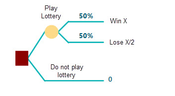
Decision tree with a 'Play Lottery' branch (fifty-fifty win X or lose X over 2) and a 'Do not play lottery' branch with payoff zero, used to elicit the certainty equivalent.

Now ask yourself: if X is $1000, would you play, knowing there is a 50% chance you lose $500? If yes, push it higher. What about $2000, or $10,000, or more? Remember that the bigger the win you name, the bigger the loss on the other side. Set X = $50,000 and you are facing a 50% chance to win $50,000 and a 50% chance to lose $50,000/2 = $25,000. Would you still play, risking $25,000 to chase $50,000? If that is your limit, then $50,000 is the number to use for R in your exponential utility function. If you would go further, say risk $100,000 to chase $200,000, then your Risk Tolerance is $200,000. In short, find the biggest X where you would still take the bet, and that is your R.

The exact way (based on the Certainty Equivalent)

So that is the fast way to guess R by answering one question from the tree above. Now let us get an exact value for R with a bit of math. This time, instead of naming the biggest winning payoff, you answer with the Certainty Equivalent of a lottery. That means you can either play a lottery with a 50% chance of winning X and a 50% chance of losing Y, or you can take a sure amount of cash instead, usually a good bit less than the lottery's top prize. That sure amount is called the "Certainty Equivalent".

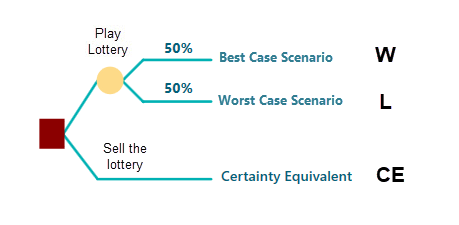
Look at the decision tree below. You have two choices. One is to play a lottery where you win "W" with a 50% chance and lose "L" with a 50% chance. The other is to take a sure amount of money and skip the lottery. Think of a friend offering to buy the lottery ticket off you. What is the least you would sell it for? Say you answer "CE". That CE is your Certainty Equivalent.

Decision tree contrasting a Play Lottery branch (fifty-fifty W or L outcomes) with a Sell the lottery branch yielding the Certainty Equivalent CE.

Now let us use the Certainty Equivalent to work out an exact Risk Tolerance for the exponential utility function.

The Expected Utility theory and the Von Neumann-Morgenstern utility theorem tell us that once you have a utility function, the Expected Utility of a gamble equals the utility of its Certainty Equivalent. That is because you only treat the two choices as equally good when their expected utilities match. Here the two choices are: play the lottery, or take a sure amount of money instead of playing.

The chances of winning and losing are both 0.5.

So let us write out the equation, where EU stands for Expected Utility.

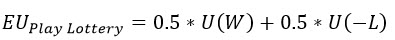
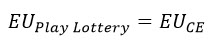
Expected utility of playing the lottery: 0.5 times U(W) plus 0.5 times U(minus L), derived from expected utility theory.

By Expected Utility theory, the expected utility of playing the lottery equals the utility of the Certainty Equivalent (CE).

Equation stating that the expected utility of playing the lottery equals the utility of the certainty equivalent, the fundamental link used to solve for risk tolerance.

Our utility function is the Exponential Utility Function, which is the one we wrote at the top of this page:

Exponential utility function U(x) equals 1 minus e to the power of negative x over R, restated before substituting into the expected-utility equality to solve for R.

So plug that function into the equation above. After simplifying, we get this:

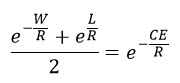
Implicit equation linking the exponential risk tolerance R, win W, loss L, and certainty equivalent CE: (e^(-W/R) + e^(L/R)) / 2 equals e^(-CE/R).

Here W is the amount you win in the lottery, L is the amount you lose, and CE is the Certainty Equivalent. All three are fixed numbers. The only unknown is R, the Risk Tolerance. To get R you have to solve this equation, and that is not a simple, one-step job. It takes a bit of work. The good news: with our Decision Analysis Software (Decision Tree Software or Rational Will) you never have to solve it by hand. The software does it and hands you the exact R. We will show you exactly how a little further down, so keep reading.

Calculating the Certainty Equivalent

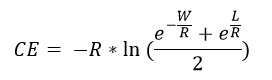
We just built an equation for finding the Risk Tolerance. The same equation also gives you the Certainty Equivalent of an exponential utility function when W, L, and R are all known. That case is easy, because the left-hand side becomes a plain number. Just take the natural log of both sides and simplify, as shown here.

Closed-form equation that expresses the certainty equivalent of a fifty-fifty lottery given an exponential utility function and its risk tolerance R.

Scaling parameters

In real life you often want the utility function set up so the best possible payoff scores the top utility value (1) and the worst payoff scores the bottom value. Adding the two parameters "a" and "b" lets you scale the exponential utility that way, like this:

So "a" and "b" come out different for each lottery or scenario.

How do you find "a" and "b"?

Say your top utility is 1. For the investment in front of you, the best possible gain is H and the worst possible gain (or loss) is L.

Then your scaled utility function, with "a" and "b", works out to:

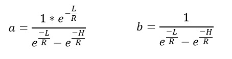
Algebraic solution for the scaling parameters a and b of an exponential utility function in terms of the highest gain H and lowest loss L.

Say a lottery can win you at most $1000 and lose you $500. Plug those numbers in and you get "a" and "b" as:

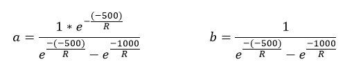
Numeric example evaluating the scaling parameters a and b for a lottery with maximum gain 1,000 dollars and maximum loss 500 dollars.

In the equation above, R is the Risk Tolerance, as before. When you use the SpiceLogic Decision Analysis Software (Decision Tree Software or Rational Will), these scaling parameters are worked out for you automatically from your other inputs.

Marginal Utility

Marginal Utility tells you how much your utility shifts when the payoff changes by a small amount. In math terms, differentiate the utility function U(x) with respect to the payoff x, and you get the Marginal Utility function.

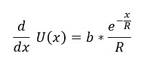
Here "b" is a scaling parameter, R is the Risk Tolerance, x is the real-life payoff, and U(x) is the utility for that payoff x.

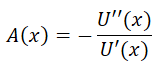
Risk Aversion

Risk Aversion is a function that tells you how risk-averse a decision-maker is, and you can derive it from the utility function. As we covered in the Utility Function chapter, the absolute risk aversion is

and the relative risk aversion is

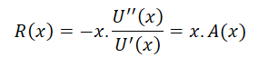
Relative risk aversion formula: minus x times U double-prime of x divided by U prime of x, applied to any utility function U(x).

Apply these to a scaled utility function and we get:

Absolute risk aversion of the exponential utility function, simplifying to the constant 1 over R, confirming exponential utility models constant absolute risk aversion.

Relative risk aversion of the exponential utility function, expressed as x over R, showing how relative risk aversion grows linearly with wealth.

Notice that the absolute risk aversion of an exponential utility function is a constant, 1/R, no matter how much wealth you have. That makes the exponential utility function a good fit for people whose attitude to risk stays the same whether they are rich or poor. Many people, though, get less risk-averse as they get wealthier, and that is the idea behind the Bernoulli Utility Function.

A worked example

Say you are thinking about a business investment. You hope it earns you $1000 over its lifetime, but you are also worried that your $200 starting investment could be lost on a 50/50 chance. Should you invest or not? You decide to use an exponential utility function to turn the money into a sense of satisfaction. Why bother? Doesn't more money just mean more satisfaction? Up to a point, yes, but more money usually comes with more risk too. You might be content once you hit a certain target, and that is exactly where a utility function earns its keep.

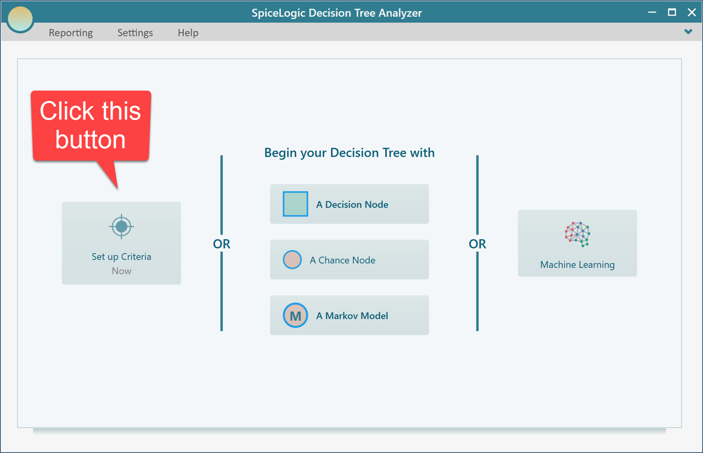
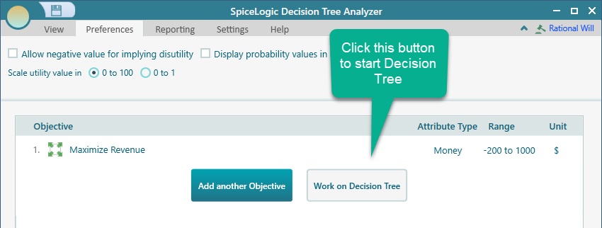
If you are using the SpiceLogic Decision Tree Analyzer, you will see the screen below. If you are using Rational Will, click the "Decision Tree" button on the home screen to reach this view. Then click "Set up Criteria".

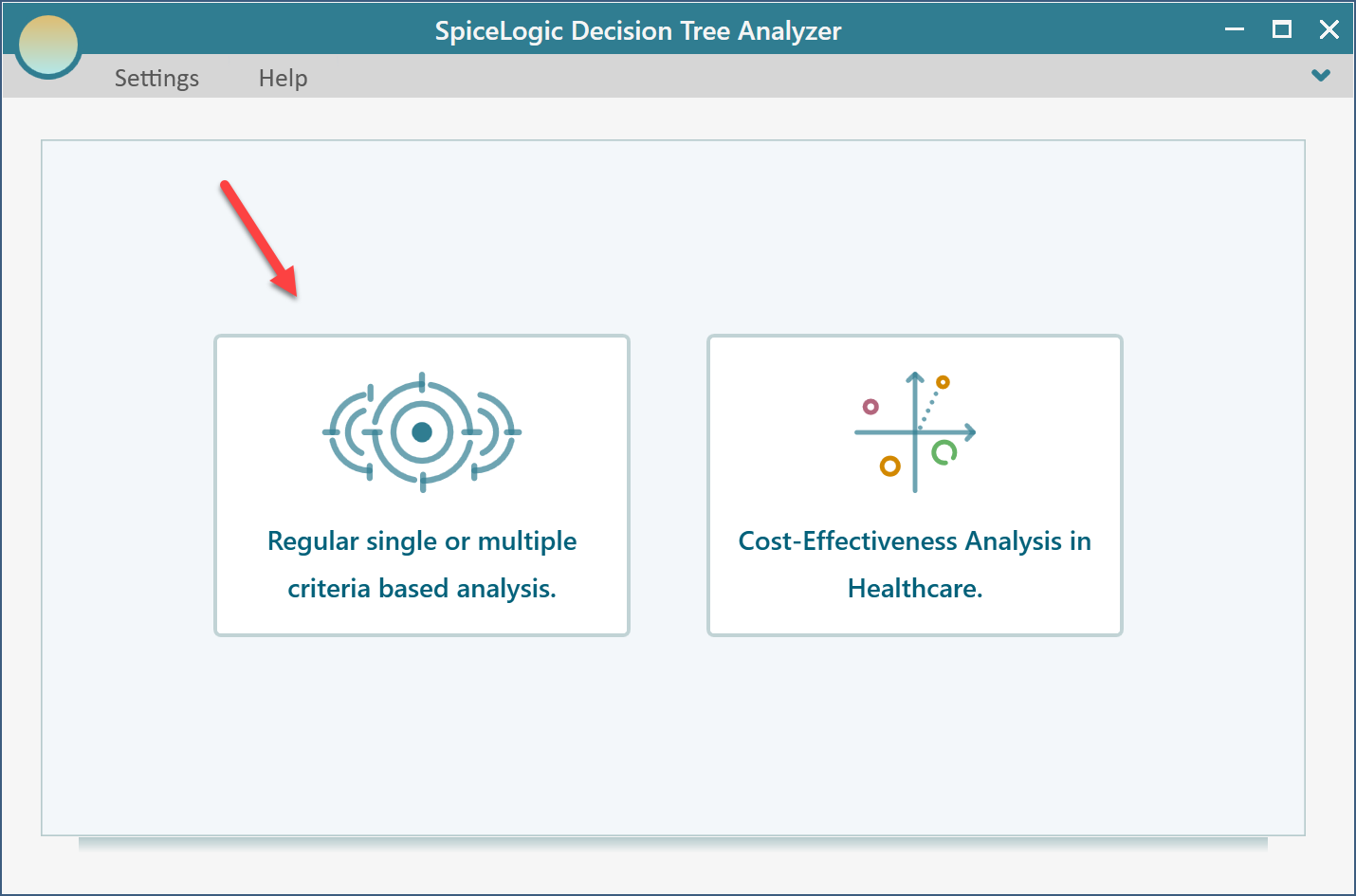
SpiceLogic Decision Tree Analyzer start page with the 'Set up Criteria Now' button highlighted as the entry point, alongside Decision Node, Chance Node, Markov Model, and Machine Learning options.

After you click that button, it asks whether you want a regular single or multiple criteria analysis, or a Cost-Effectiveness analysis. Pick the first option.

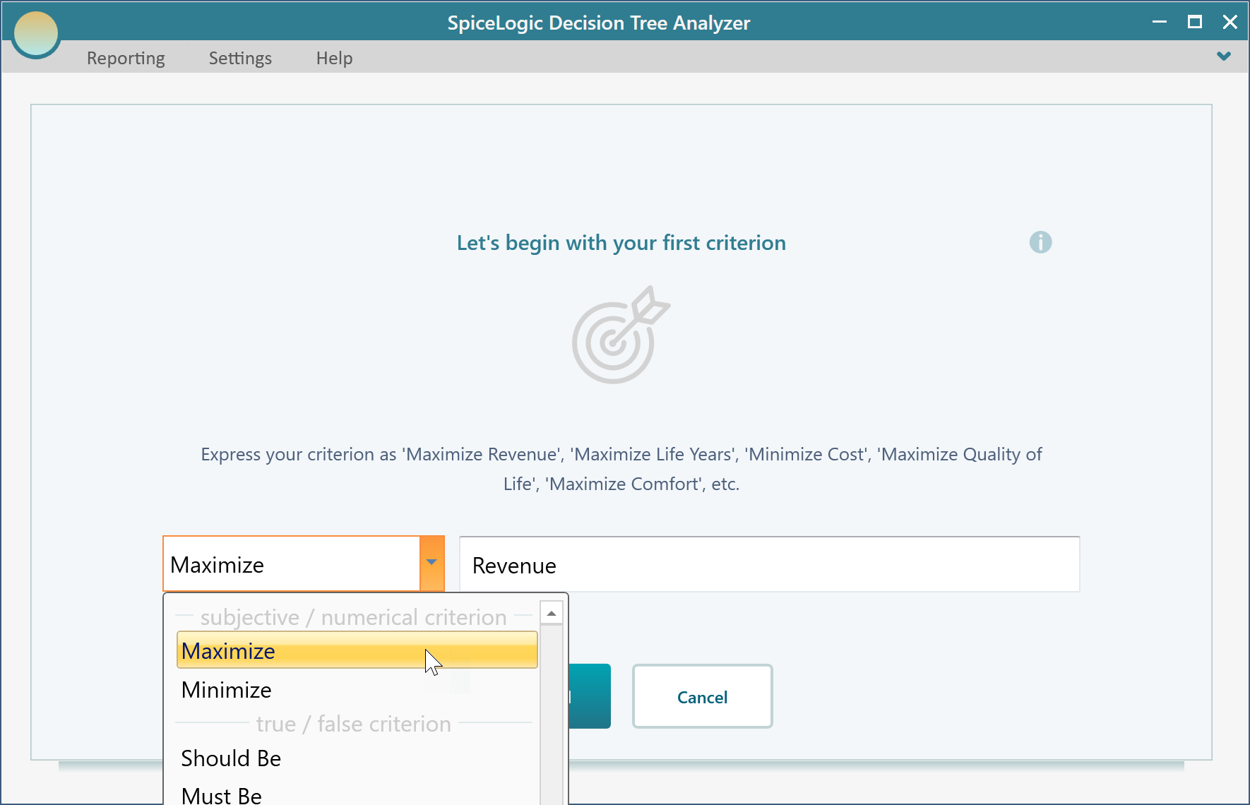
Payoff type selection dialog asking the user to choose between regular single or multiple criteria analysis and a cost-effectiveness analysis.

Next you will see the screen below. Choose "Maximize" and type in "Revenue", as shown.

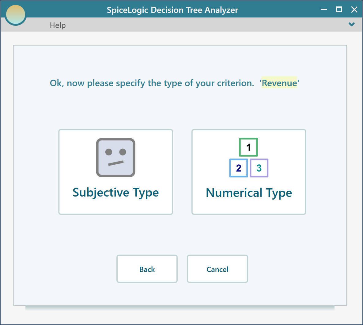
Criterion setup screen with Maximize selected and 'Revenue' entered as the objective name for the new decision tree analysis.

Then click "Proceed". It asks for the type of criterion. Choose "Numerical Type". Keep in mind that you can only use a utility function with a Numerical type criterion.

Criterion type selection dialog offering Subjective Type or Numerical Type for the Revenue criterion; the Numerical Type is required to attach a utility function.

Next it asks for the smallest and largest payoff the investment could produce. Enter Minimum = -200 (since you could lose your $200 investment) and Maximum = 1000.

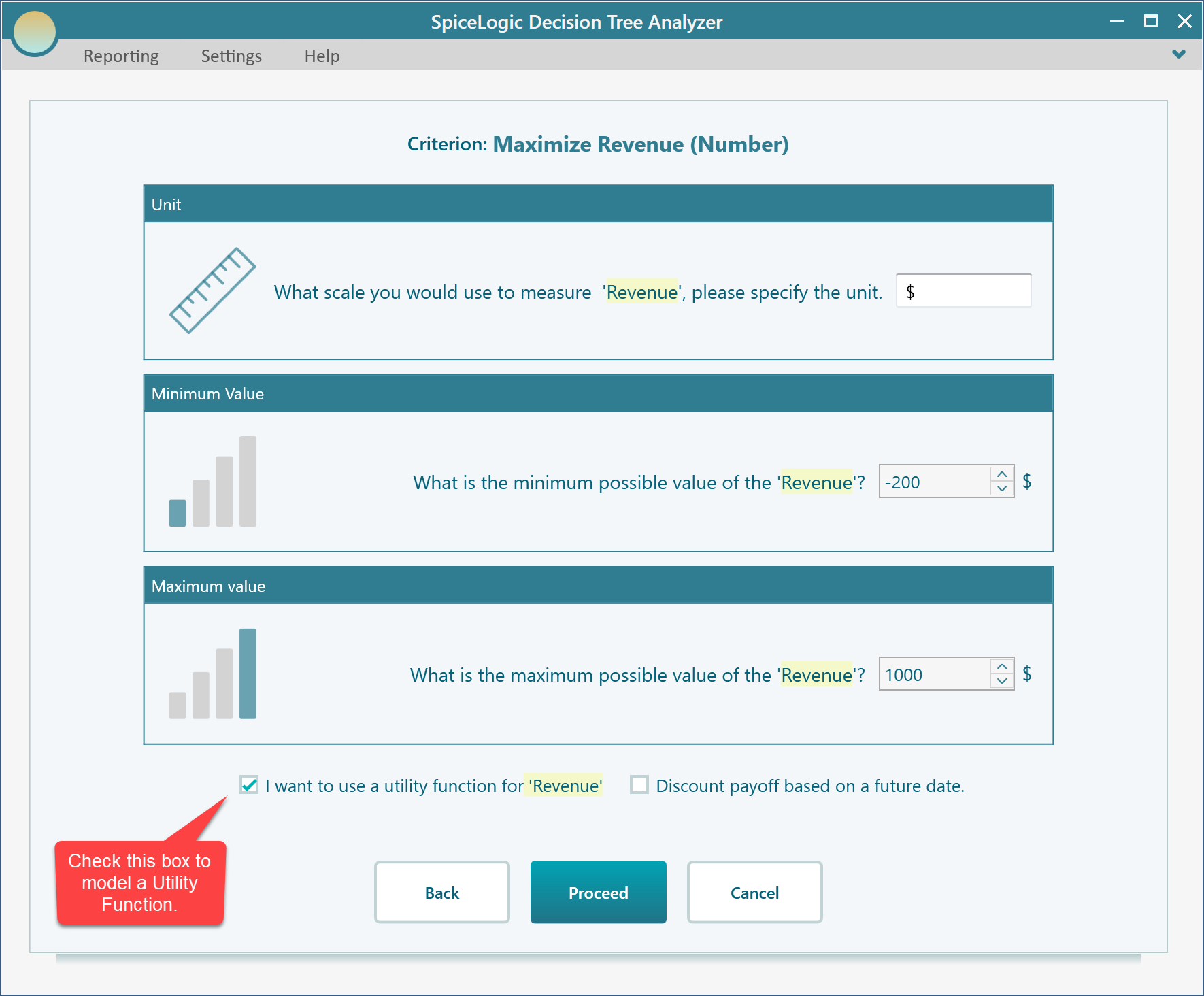
Numerical criterion details for Maximize Revenue: unit dollar, minimum value minus 200, maximum value 1000, with the 'I want to use a utility function' checkbox ticked.

Click Proceed. Because you ticked the box "I want to use a utility function...", a utility function editor opens. Click the "Exponential Utility Function" button.

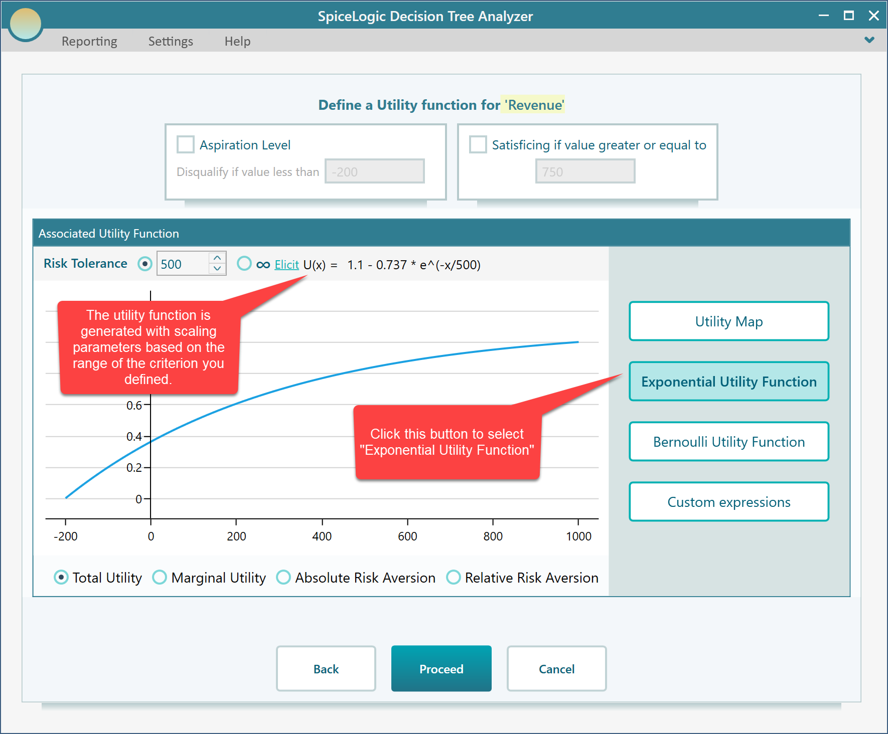
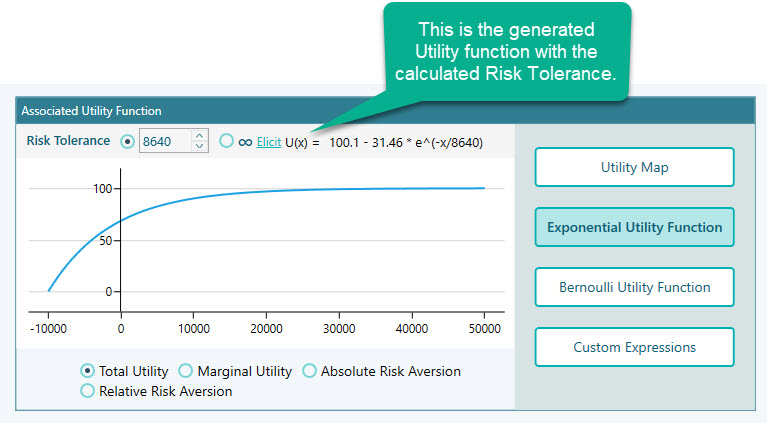
Utility function editor in Decision Tree Analyzer with the Exponential Utility Function button highlighted, ready to auto-generate the curve with calculated scaling parameters.

In the screenshot above, you can see an exponential utility function has been built for you, with the scaling parameters already worked out.

How the scaling parameters are calculated

You might wonder where the scaling values 109.98 and -73.72 in that function come from. They are chosen so the best payoff lands on the highest utility value, which can be 1 or 100 depending on your preference, and the worst payoff lands on the lowest value, which can be 0, -1, or -100, again depending on your preference. You set this preference from the ribbon, as shown here.

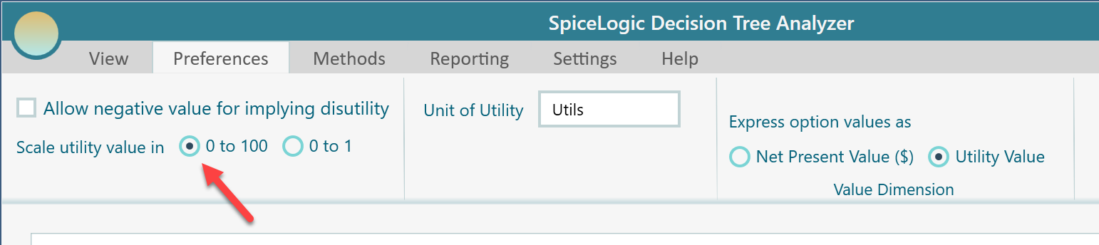
Preference unit selector inside the utility function editor with the 0 to 100 scale chosen for the exponential utility examples.

Let us set the utility scale to run from 0 to 100. The choice is yours, but the examples below all use the 0 to 100 range.

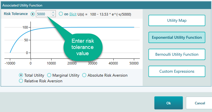
Setting the Risk Tolerance

The key parameter in the exponential utility function is Risk Tolerance. You can type the Risk Tolerance value straight in here, as shown in the screenshot below.

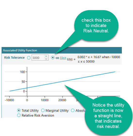
Risk Tolerance input field in the Exponential Utility editor where the user can type R directly to control the concavity of the utility curve.

If you are completely risk-neutral, your Risk Tolerance should be infinity. You can set that by clicking this radio button.

Risk-neutral utility function plot produced by selecting the infinite Risk Tolerance radio button, yielding a straight line through the payoff range.

Working out your Risk Tolerance

As we explained earlier, there are two ways to find the Risk Tolerance R of an exponential utility function: the approximate way and the exact way. The approximate way is easy to grasp and use, but since you have the software in front of you, why not start with the exact way and let it do all the hard math for you?

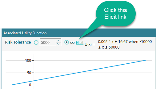
The exact way

To use the exact way to find your Risk Tolerance, click the "Elicit" link, shown below.

Link in the Exponential Utility editor that opens the risk-tolerance elicitation window, offering both the exact and the approximate elicitation methods.

Click that link and the window below opens, with the "Exact Risk Tolerance" method already selected. You will see a decision tree filled in for you, with the Best Payoff set to the criterion's maximum and the Worst Payoff set to its minimum, the two numbers you entered earlier. You can change them with the sliders if you like. Once the Best Payoff and Worst Payoff are set, use the slider to enter a Certainty Equivalent value. The Risk Tolerance is then worked out and shown right away.

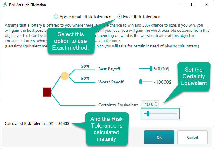
Exact Risk Tolerance elicitation window in Decision Tree Analyzer showing a pre-populated decision tree where the user enters their certainty equivalent for the lottery.

Click OK and the calculated Risk Tolerance is carried back into the exponential utility function editor.

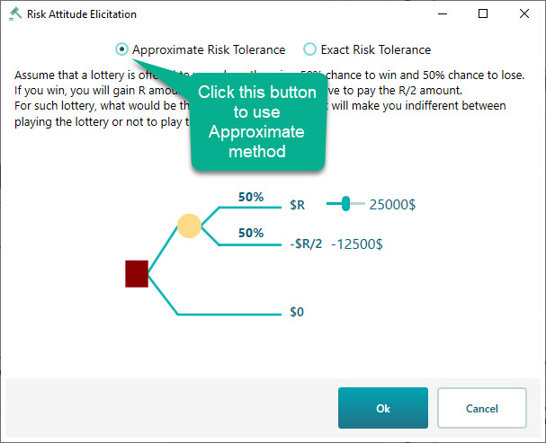
Auto-generated exponential utility function in the editor after the elicited risk tolerance was passed back from the elicitation dialog.

The approximate way

You can also try the approximate way to find your Risk Tolerance R. Click the "Approximate Risk Tolerance" radio button, shown in the screenshot below. There you will see a decision tree where the winning amount is set to the criterion's maximum value that you entered, and the losing amount is filled in automatically as half of the winning amount. Use the slider to think about the biggest winning number you would still play for, knowing there is a 50% chance of losing half of it.

Approximate Risk Tolerance elicitation window in Decision Tree Analyzer using a simpler decision tree to derive R without solving the exact equation.

Looking at other versions of the generated utility function

Beyond the exponential utility function itself, you can also view several related versions of it in the Decision Analysis software (Decision Tree Software or Rational Will). At the bottom of the chart you will find a set of radio buttons, shown in the screenshot below. Click "Marginal Utility", for example, and you will see the Marginal Utility function equation along with its plot, like this.

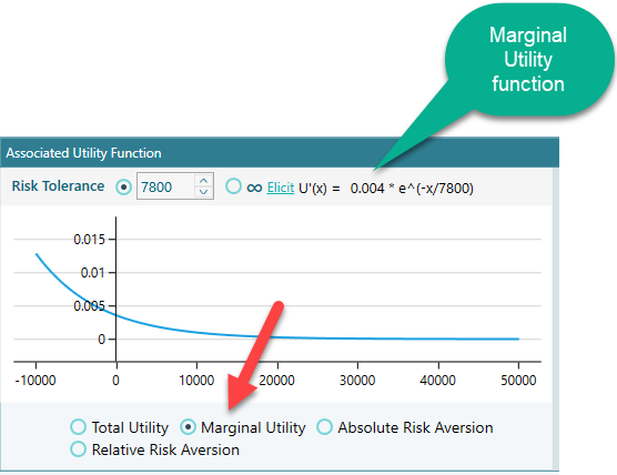
Marginal Utility Function view in the utility function editor, selected via the bottom radio buttons that also expose absolute and relative risk aversion plots.

You get a similar view for Absolute Risk Aversion and Relative Risk Aversion too.

Now build the decision tree

When you are happy with your utility function, click OK in the Objective editor. That takes you to the Objectives manager page. Click the "Work on Decision Tree" button.

Objectives list page with Maximize Revenue defined and the 'Work on Decision Tree' button highlighted, used to proceed to the tree designer after configuring the utility function.

Then click the "Decision Node" button to start your decision tree with a decision node.

Decision Node button on the decision tree start screen, used to create a tree whose root is a decision node.

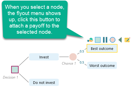
Now build a decision tree like the one shown. If you are new to building decision trees in our software, take a look at the getting started page, which shows you how to set a payoff on a node.

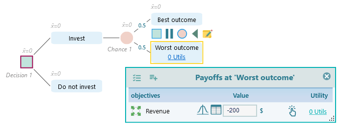
Sample investment decision tree with 'Invest' and 'Do not invest' branches under the root decision node, used in the exponential utility worked example.

Set a payoff of $1000 for the Best outcome, -$200 for the Worst outcome, and 0 for the "Do not invest" node.

Once every node payoff is set, the decision tree will look like this.

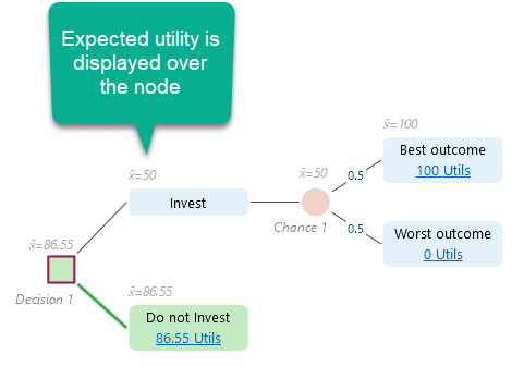
Final decision tree after all node payoffs were set, with utility values calculated by the exponential utility function shown on each node.

Note that the numbers shown in utils on the tree nodes are the calculated utility values. You enter the real payoff and the software works out the utility from your utility function. For example, the "Do not Invest" node shows 86.55 utils. Why? Because in the exponential utility function we built, a payoff of 0 maps to a utility of 86.55, and the real payoff for "do not invest" is 0. For the Worst outcome node we entered -200, which came out as 0 utility, and for the Best outcome node we entered 1000, which came out as 100 utils under the generated function.

Notice too that the Expected Utility is calculated and shown above the node. The "Invest" node shows an expected utility of 50 utils, which is lower than the 86.55 of "Do not invest", so the "Do not Invest" node is highlighted in green to mark it as the recommended choice.

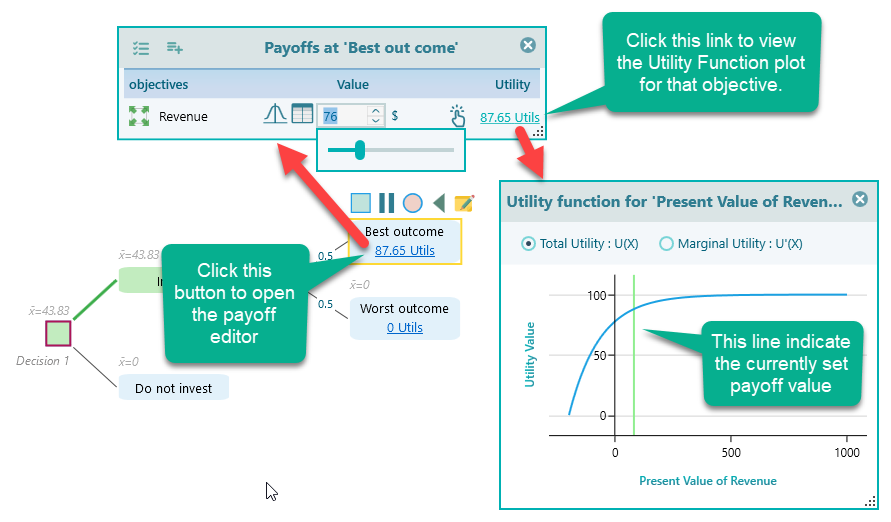
Click the Utils link on any node and the payoff editor opens. There you can see the payoff and the utility function plot, with a green vertical line showing where your utility sits for the current payoff. Move the payoff and the line moves with it, right away.

That is it. We hope you enjoy using the Decision Analysis software (Decision Tree Analyzer or Rational Will) to model your exponential utility function.