Various Risk Metrics

The Decision Tree software gives you a wide set of metrics for any tree you build. You are not stuck with one number. You pick the metric you care about right now, and the software shows it to you in the Options Analyzer carousel. That way you can study the same tree from a few different angles instead of just one. Say you have built the decision tree shown below.

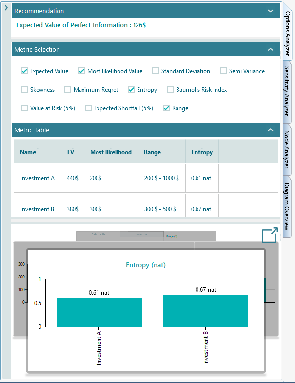
When you expand the Options Analyzer tab, you will see that you can pick from many metrics. Whatever you choose shows up in both the chart and the metric table, side by side. So you can read the exact numbers and see their shape at the same time.

The list of metrics changes to fit the tree you have. The software only shows the metrics that make sense for your decision. For example, if your tree has no uncertainty in it, meaning no chance node, then the metrics about risk and uncertainty simply will not appear in the metric selection panel. There is no point offering a risk number when there is no risk to measure.

Most of the time, these are the metrics you can choose to show in the metric table and the chart carousel.

Expected Value

The expected value is the average outcome you would get if you could repeat the same decision over and over, with each possible result weighted by how likely it is. It is the most common way to sum up an uncertain payoff in a single number. The software works it out with the formula below.

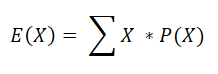
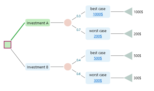
Here X is a random variable that stands for each possible outcome, and P(X) is the probability of that outcome. In plain words, you multiply each outcome by its chance of happening, then add them all up. For example, take the decision tree below.

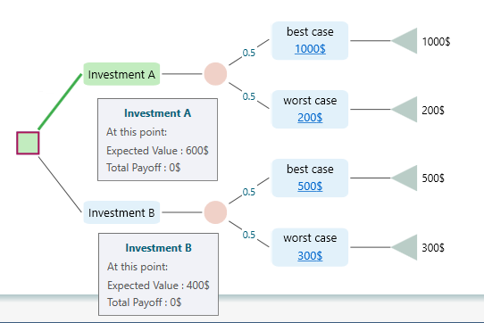
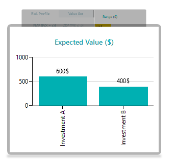
The expected value of Investment A is EV = 0.5 * 1000$ + 0.5 * 200$ = 600$. There is a half chance of getting 1000$ and a half chance of getting 200$, so on average you would expect 600$. The expected value chart shows it like this.

Most Likelihood Value

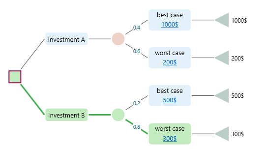
The most likelihood value is simply the outcome most likely to happen, the one with the highest probability. In the decision tree below, the most likely value for Investment B is the Worst Case outcome. That may sound odd at first, but it makes sense once you look at the chance node. The Worst Case has a probability of 0.8, which is higher than any other event in that node. So even though it is the worst result, it is also the one you are most likely to actually get.

Standard Deviation

Standard deviation tells you how spread out the possible outcomes are. A small number means the results sit close together. A large number means they are all over the place.

Here is a simple example. In class A, four students score 50, 58, 55, and 52. Those scores are clearly close together, so the spread is low. In class B, four students score 10, 100, 70, and 40. Those scores are all over the place, so the spread is high. The average for class B is 55 and the average for class A is 53.75. If you only looked at the averages, you might think class A is doing a bit worse. But the averages hide the real story. Class A is steady, and every student performs at about the same level. Class B has one student barely passing and another acing it. If consistency matters to you, the average alone gives you the wrong picture. You need a number that tells you how spread out the values are, and that number is the standard deviation.

When outcomes are uncertain, we call the outcome a random variable. The standard deviation of a random variable X is usually written as σ or σ_x.

For a discrete random variable, the standard deviation is worked out with the formula below.

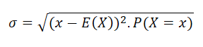
Here x is a possible outcome, P(X = x) is the probability of that outcome, and E(X) is the expected value. In short, you measure how far each outcome sits from the average, weight that by its probability, and combine it all into one number.

Semi-Variance

Standard deviation treats good surprises and bad surprises the same way. But often you only care about the downside, the chance of falling below a level you would be unhappy with. Semi-variance measures exactly that: the spread of the bad outcomes only. Think of an investor who is fine with any return above what they put in, but loses sleep over anything below it. Standard deviation would count a big gain as risk too, while semi-variance ignores the upside and looks only at the part that hurts. The formal definition is below.

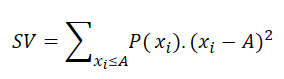
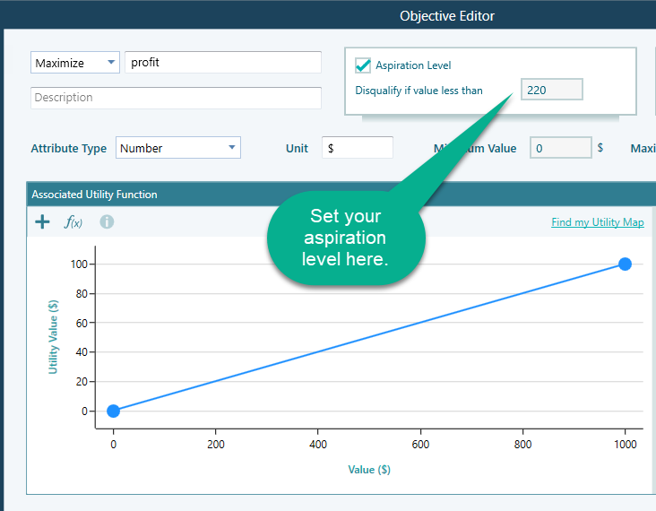
Here x_i is a possible outcome and P(x_i) is the probability of that outcome. A is a threshold you set. Any payoff below A counts as a failure, and only those below-A outcomes go into the measure. For example, you might have a salary you need to hit when choosing a job. If a job pays less than that amount, you would not even consider it. That cut-off line is your aspiration level. To set it in the Decision Tree software, open the Payoff popup and double-click the Criteria to open the objective editor.

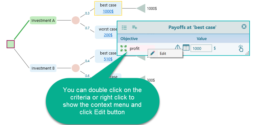
Once the objective editor is open, you set your aspiration level like this.

A few things to keep in mind:

1. The aspiration level can only be set for Number and Monetary type objectives.
2. If you do not set an aspiration level, the software falls back to using the Expected Value as the threshold, and the semi-variance is worked out against that.
3. If you have more than one objective, each one could have its own aspiration level, so there is no single threshold to base one semi-variance on. In that case the software again uses the Expected Value (or Expected Utility) as the aspiration level and works out the semi-variance from there.

Maximum Regret

Maximum regret answers a simple worry: if you pick this option, how much could you kick yourself later for not picking a different one? It looks at the worst case where another choice would have served you better, and measures that gap. So if you chose Option A and earned 200$ while Option B would have earned 900$, your regret for that case is 700$. The full explanation is on the Decision Criteria page.

Baumol's Risk Measure

William Baumol proposed the following risk index.

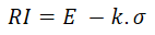
Here E is the expected value, σ is the standard deviation, and k is a constant chosen by the investor that reflects how much safety they want, that is, a level the return is unlikely to fall below. In the Decision Tree software, k is worked out from a value you provide called the significance level. This is the same significance level used in the Value at Risk calculation.

Chebyshev's inequality:

The probability of a payoff below E - k.σ is no more than 1/k².

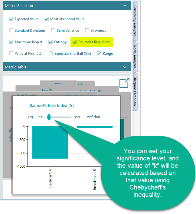
So the value of k can be worked out from the significance level. When you pick the Baumol's Risk Measure metric, the software asks you for your significance level α right there in the carousel.

Roy's safety first rule

A. D. Roy started from a plain idea: investors mostly want to avoid disaster. So instead of measuring spread, he measured the chance that the outcome ends up below a level you would call a bad result, your aspiration level. The lower that chance, the safer the option looks. Roy's risk index is defined as follows.

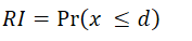
Here 'd' is the aspiration level. In the Semi-Variance section above, we showed how to set the aspiration level for an objective, and the same setting is used here.

Once you have set the aspiration level, the metric Roy's safety first rule becomes available in the metrics panel.

Entropy

Think about watching a movie. If you can guess every twist before it happens, there is no suspense and the movie falls flat. So how would you measure that suspense? You would say the harder a thing is to predict, the more suspense you feel.

That is the idea behind entropy. Entropy measures how hard it is to predict the outcome of a random variable. Probability tells you how likely a single outcome is. Entropy tells you how uncertain the whole thing is, in other words, how much surprise is built into it. A uniform probability distribution has the highest entropy, because every outcome is equally likely and you can never guess what comes next, so you stay in suspense the whole time. A normal distribution is different. Outcomes cluster around the mean and are fairly predictable, so a normal distribution has lower entropy than a uniform one.

Building on Boltzmann's H-theorem, Shannon defined the entropy H of a discrete random variable X as follows.

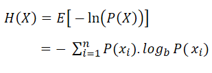
Here b is the base of the logarithm. In the Decision Tree software you can switch the base between e, 2, and 10 by changing the unit to nat, Shannon, or Hart.

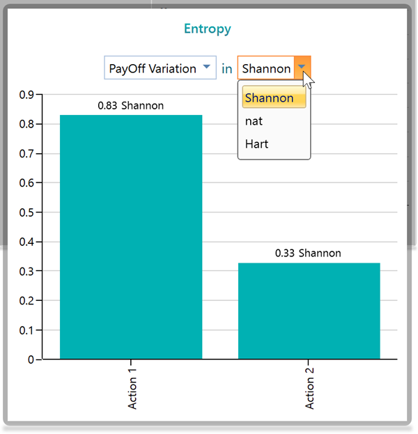
You will also notice a dropdown in the Entropy chart panel.

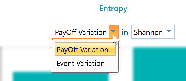
What do these options do? To see it clearly, look at the decision tree below.

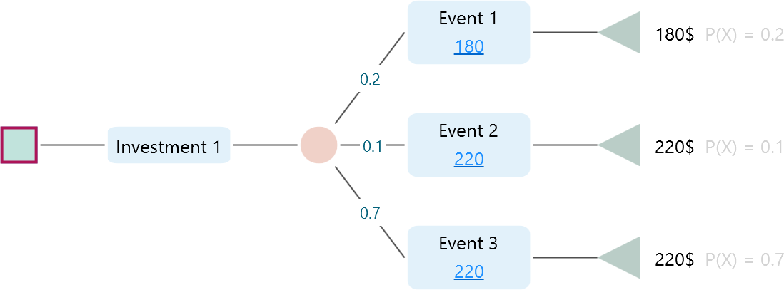
In this tree, Investment 1 has three events, but two of them lead to the same outcome, 220$. So if all you care about is the actual money you walk away with, there are really only two different results, 180$ or 220$, not three. If you pick "Payoff Variation", the software groups events by their final outcome and treats two events as the same when the payoff is the same. By that count there are two outcomes here, and the entropy is worked out on that basis. But say you do not care about the final payoff and instead care about how many separate events could happen. Then there are three. Pick "Event Variation" and the software works out entropy treating all three as distinct outcomes.

Let's look at the result in the Entropy panel.

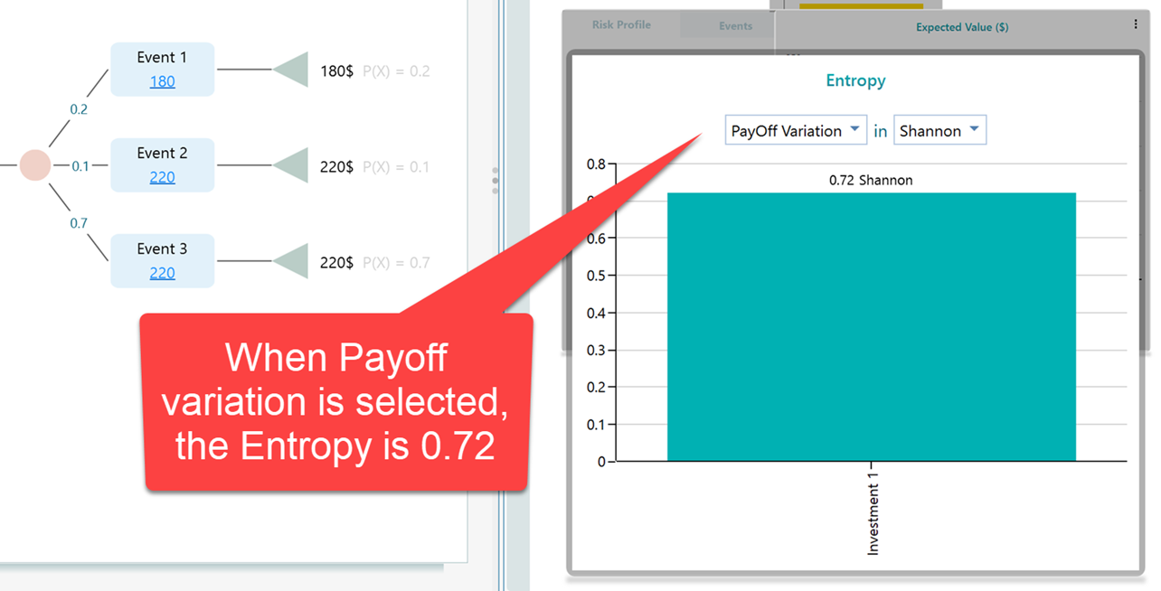
With two outcomes (Payoff Variation), the entropy comes out to 0.72 Shannon. Now let's switch the dropdown to Event Variation.

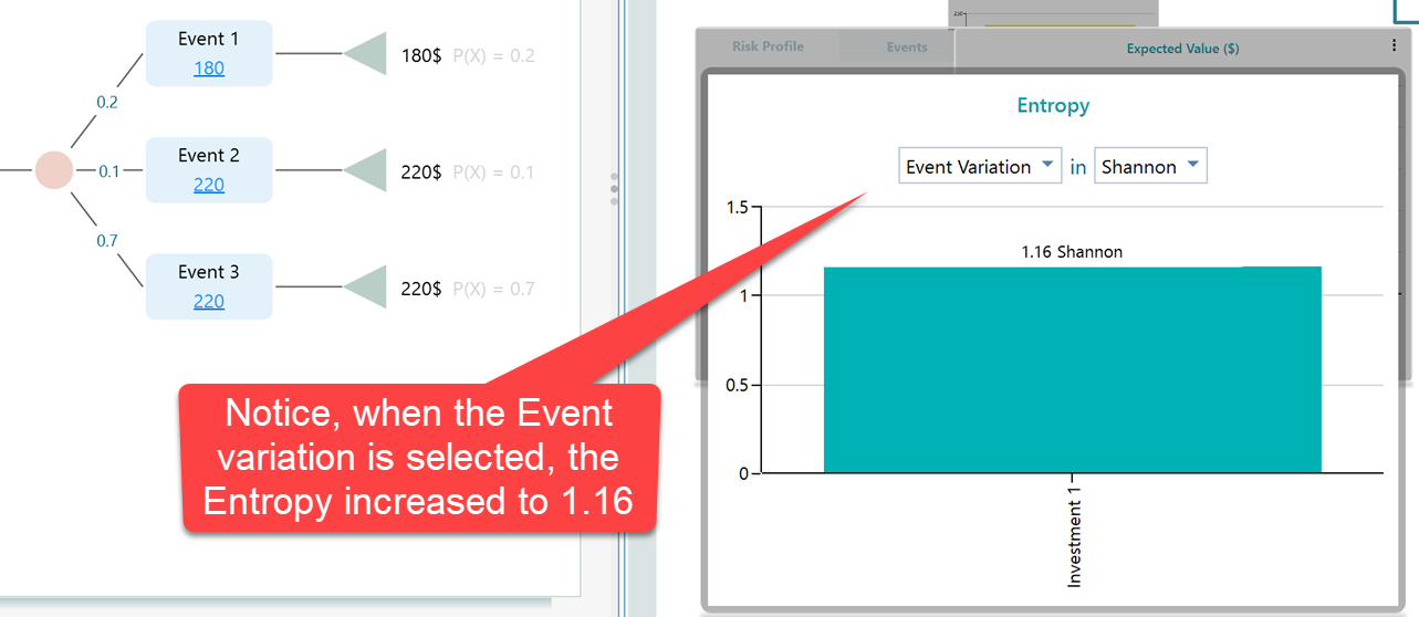
This makes sense. When you only had two possible outcomes, things were easier to predict. You knew it would be either 180$ or 220$, so there was less suspense. With Event Variation, outcomes are counted by the name of the event rather than the final payoff, which gives you three outcomes here. Three possibilities are harder to predict than two, so naturally the entropy, the suspense, is higher.

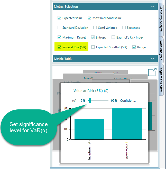
Value at Risk

Value at Risk, written as VaR(α), is a risk number used widely in practice, especially by banks and other financial firms. It tells you the most you would expect to lose at a chosen confidence level. For example, it answers a question like "with 95% confidence, what is the worst loss I should plan for?" In the Decision Tree software you can turn on the Value at Risk metric from the metrics panel. The chart in the carousel then lets you set your confidence level, or significance level (α), as shown below.

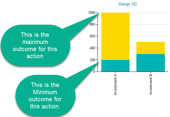
Range Chart

A range chart shows the lowest possible value and the highest possible value of an option as a single band. With one glance you can see how far down things could go and how far up, which gives you a quick feel for both the risk and the upside. From there you can compare options using the Maximin or Leximin criterion, picking the option whose worst case is the least bad. The range chart also makes it easy to spot dominance. When one option's whole range sits above another's, it dominates that option, either outright or in a stochastic sense.