Markov Models - Life Expectancy with Time variant probability

This example walks through a question many people ask: on average, how long does a group of people live when the chance of dying changes with age? That average is called life expectancy. A Markov Chain fits this well, because life can be seen as a series of yearly steps. At each step a person is either still alive or has died.

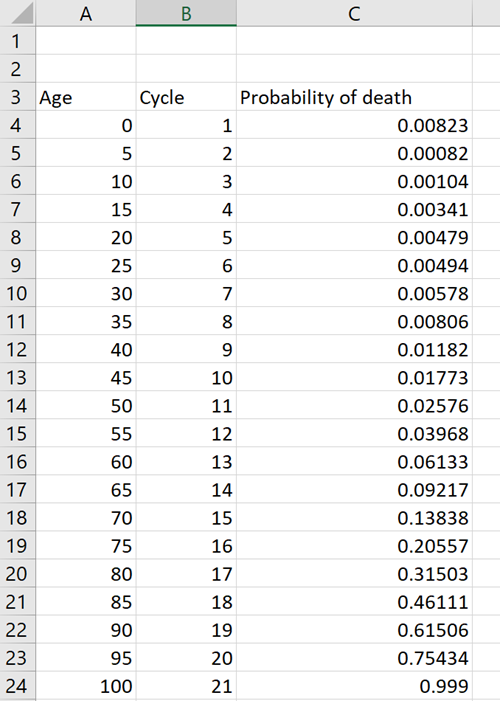
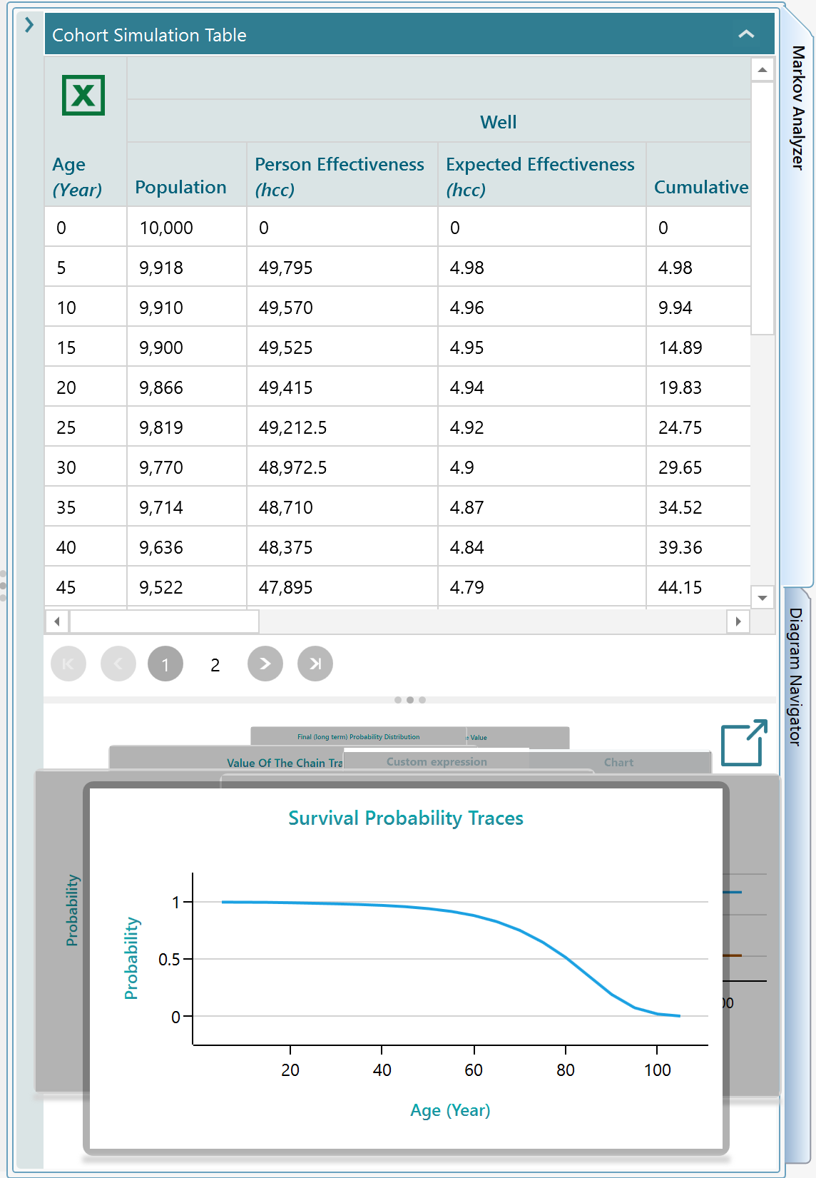
Say we start with a group of 10,000 people. We know the chance of death at each age, from year 0 to year 100. You can see those numbers in the table below. The chance of dying is small in early adulthood and climbs steadily in old age. So one fixed number will not work for a whole life. The chance depends on how old the person is right now. The rest of this guide shows how to build the model and read the answer, one step at a time.

Sample data table for the life expectancy example, mapping age in years (0 to 100) to the probability of death used as the time-variant Markov transition.

Open the Rational Will or the Decision Tree software. On the start screen, choose "Markov Model".

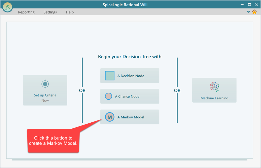
Decision Tree Analyzer start screen with the Markov Model button highlighted, used to begin the life expectancy Markov chain example.

We pick a Markov node as the root of the Decision Tree because this example is only about the Markov Chain, not a bigger decision. Starting this way keeps the model simple. If you want to compare options later, that is fine. Once the model is built, you can add decision nodes on top of it and do more analysis. After you make this choice, a wizard opens that looks like this:

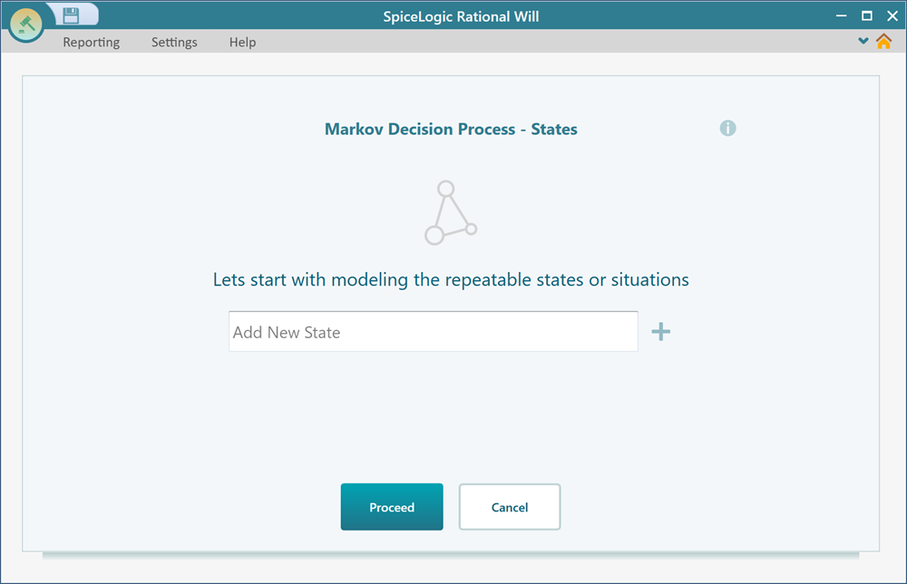
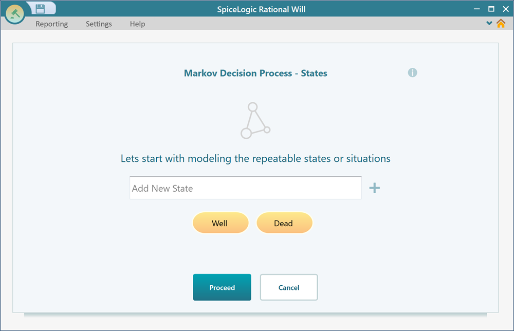
Opening screen of the Markov Model wizard launched after choosing a Markov node as the root of the tree for the life expectancy example.

Step 1: Creating the Markov States

A Markov state is just a situation a person can be in. For this model there are only two: being alive, and being dead. In the wizard, add two states and name them "Well" and "Dead". Then click Proceed.

Markov wizard step 1 with two states named Well and Dead added to the chain for the life expectancy cohort model.

Next, the wizard asks you the following question.

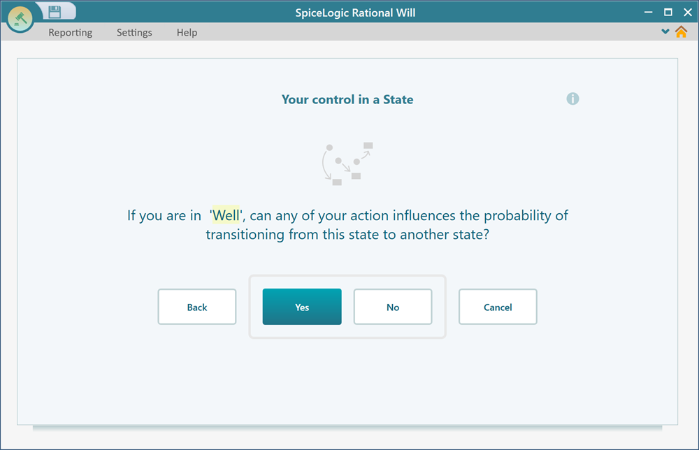
Wizard prompt 'Your control in a State' asking whether the user's actions can influence the probability of transitioning from the Well state to another state, with Yes / No / Back / Cancel options.

In plain terms, it is asking whether you want to use an Action in your Markov Model. An Action is a choice you control, like starting a treatment. This model has no actions, only states (Well and Dead), so click No. The wizard then asks the same question for the "Dead" state. Answer No there as well.

Step 2: Setting up the Markov Simulation

After you answer No, the wizard moves on to the simulation settings. A Markov Model is solved by running a cohort simulation. That means the software follows the whole group of 10,000 people forward in time, cycle by cycle, and counts how many are still alive at each step. Here you decide how that run works.

For this example, turn on Half Cycle Correction by checking that box. Half Cycle Correction is a small accuracy fix. People who die during a cycle do not all die at the very end of it, so this evens out the timing and gives a more realistic result. Set the number of iterations to 21 and the duration of each cycle to 5 years. That gives you 21 steps of 5 years each, which covers the full age range we care about. Set the Cohort Size to 10,000. The cohort size does not change the answer by much, but a larger group gives a smoother, more accurate result, and 10,000 is plenty here.

Cohort simulation settings step in the wizard with cycle count, cycle name, and cohort size configured for the life expectancy run.

Now click "Proceed".

Step 3: Setting the transition probabilities (importing from Excel)

The wizard now asks you to set the transition probabilities. A transition probability is the chance of moving from one state to another in a single cycle. For example, the chance that someone who is Well this cycle becomes Dead by the next one. This is where the age-based death rates from our table come in.

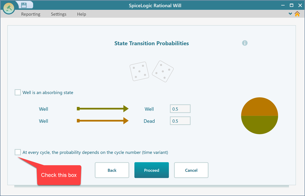
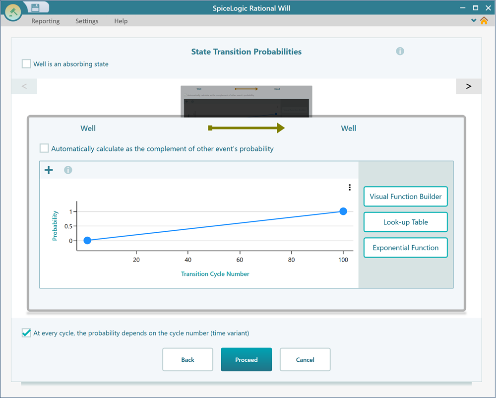
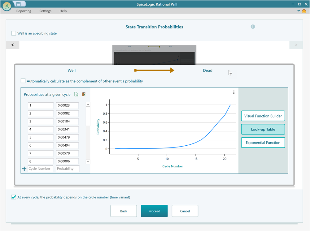
Transition probability step with the 'At every cycle, the probability depends on the cycle number (time-variant)' checkbox available for age-driven probabilities.

In our case the chance of dying is not the same every cycle. It depends on how old the group is, so the chance changes from one cycle to the next. To handle this, check the box "At every cycle, the probability depends on the cycle number (time-variant)", as shown in the screenshot above. After you check it, the wizard shows the screen below. This is a carousel that lets you page through every possible state transition, one at a time.

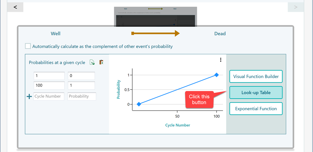
Carousel view of time-variant transition probabilities, letting the user step through each from-to state pair to configure its cycle-dependent probability.

In the carousel, find the transition for Well to Dead. If the box "Automatically calculate as the complement of other event's probability" is checked for the Well to Dead transition, uncheck it. You are turning that off because you will supply the death chances yourself from your own data, instead of letting the software work them out from the other transitions.

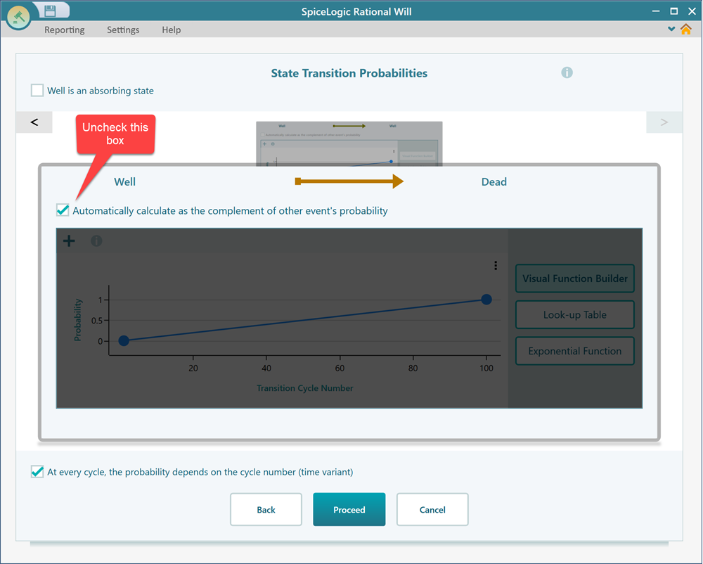
Well to Dead transition view with the 'Automatically calculate as complement' checkbox cleared so the probability can be specified directly from the data.

Now click the "Look up table" button. A lookup table view opens, where you can enter a different chance for each cycle number. Typing 21 values by hand is slow and easy to get wrong, so the next steps show how to paste them straight from Excel.

Look-up table view for the Well to Dead transition, with columns for cycle number (age) and the corresponding probability value.

Open your Excel file. Select two columns. The first column holds the cycle number, and the second column holds the matching chance of death for that cycle. With both columns selected, copy the data to your clipboard.

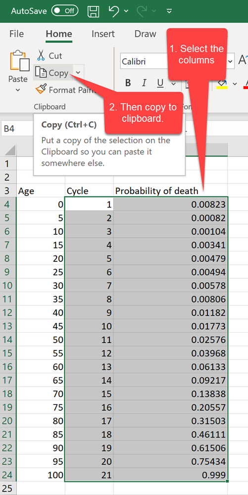
Excel worksheet with the age (cycle number) column and corresponding probability column selected and copied to the clipboard for import.

Go back to the Decision Tree software and click the button to import the table from your clipboard. Before you import, double-check that your data is laid out exactly as shown in the screenshot above: cycle number in the first column, chance of death in the second. If the columns are in the wrong order, the values will line up incorrectly.

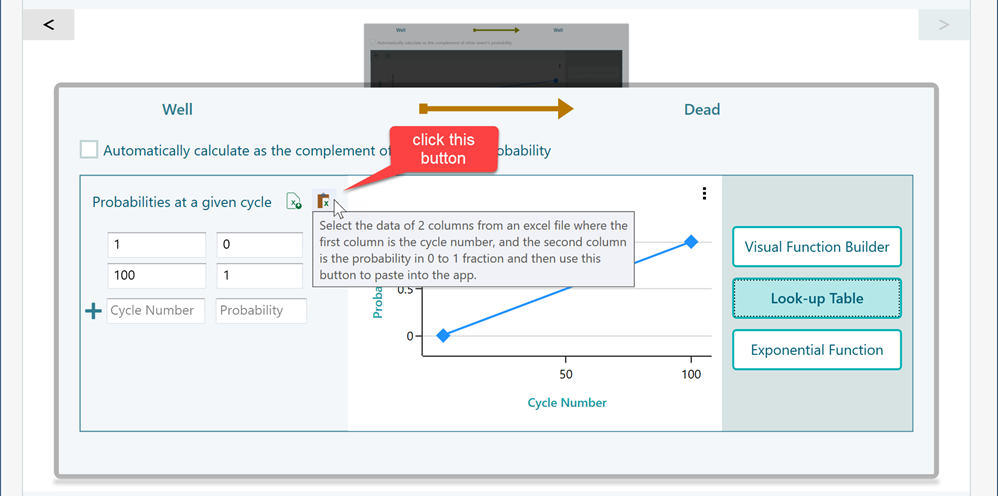
Import-from-clipboard button on the look-up table editor used to paste the age and probability columns previously copied from Excel.

After you click the import button, the data appears in the lookup table as shown below.

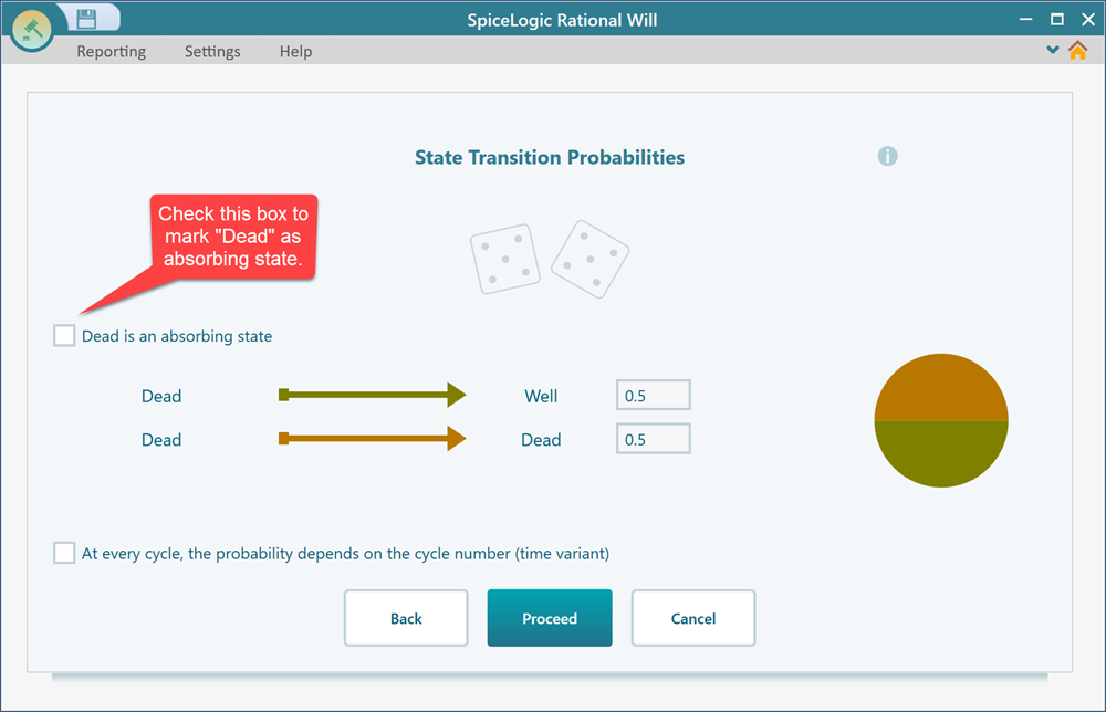
Look-up table populated with age-to-death probabilities imported from the Excel clipboard, ready to drive the time-variant Markov transition.

Now click "Proceed". The wizard then asks you to set the transition probabilities for the "Dead" state. Death is an absorbing state. That means once someone is dead, they stay dead. There is no chance of moving from Dead to any other state, so every transition out of it is 0. To capture this, check the box that says "Dead is an absorbing state".

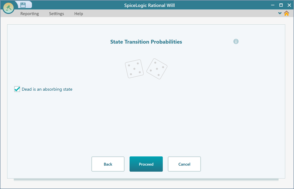
Transition setup for the Dead state with the 'Dead is an absorbing state' checkbox enabled so no transition can leave Dead in the simulation.

Once you check that box, the transition probability controls disappear, because there is nothing left to set for an absorbing state. Now click Proceed.

Transition controls hidden after the Dead state is marked absorbing, confirming the wizard accepted the absorbing-state configuration.

Step 4: Setting the Initial State

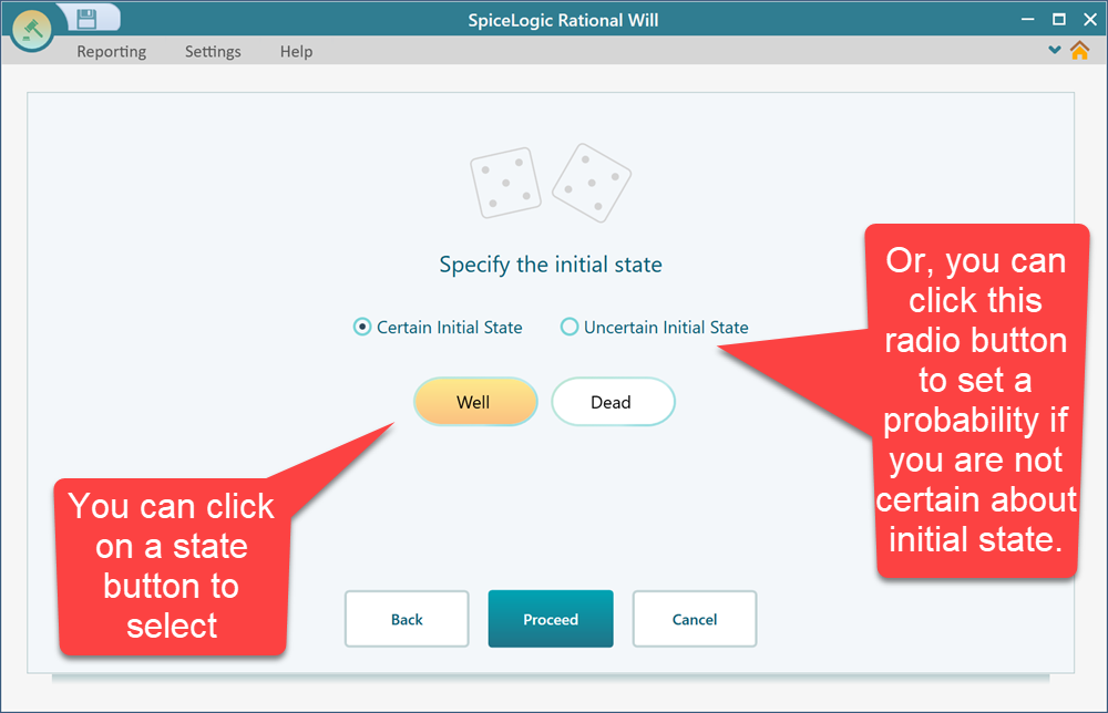
After you click Proceed, the wizard asks you to set the starting point of the group. You have two choices. You can set a certain initial state, where everyone begins in the same state. Or you can set an uncertain initial state, where the group is split across states by probability at the start. For example, if you knew 5 percent of people were already sick on day one, you would use the uncertain option to put them in a different state.

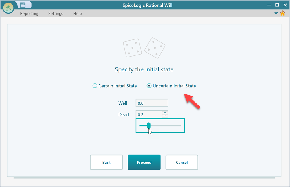
Wizard step for choosing either a certain initial state or a probability distribution across states for where the cohort starts.

The screenshot below shows what the screen looks like if you choose an uncertain initial state.

Uncertain initial state view showing per-state probability inputs that sum to 1 when the cohort does not start in a single known state.

For our model, switch back to a certain initial state and set it to "Well", since everyone in the group starts out alive.

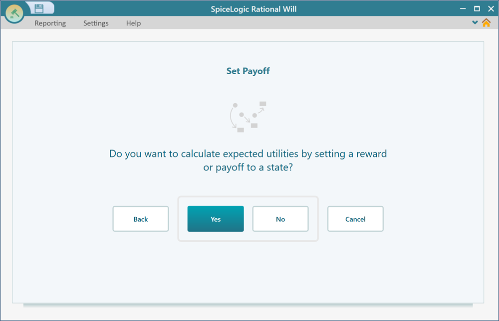
Step 5: Setting the Payoff or Reward

After you click Proceed, the wizard asks whether you want to set a payoff for your states. A payoff (also called a reward) is the value the group earns for spending time in a state. In our case the answer is yes, and the payoff is life years. Each cycle the group spends in the "Well" state is 5 years of life gained, because each cycle is 5 years long. Adding these up across all cycles is what gives us life expectancy at the end. Click "Yes" on the screen below.

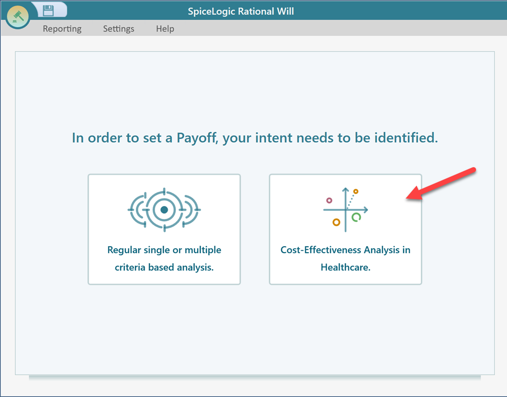
Wizard prompt asking whether to attach a payoff to the Markov states, answered Yes so a life-year reward can be added to the Well state.

Now choose the "Cost-Effectiveness Analysis in Healthcare" button. This option is built for exactly this kind of problem, where the reward you care about is measured in life years.

Objective type selection step in the wizard with the 'Cost-Effectiveness Analysis in Healthcare' button highlighted as the payoff framework.

The cost-effectiveness setup window then appears.

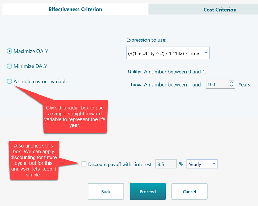
Cost-effectiveness setup window with the custom variable radio option selected to define a domain-specific effectiveness measure.

When you check the radio button for a custom variable, you can define your own reward variable, as shown below. Here that variable is the life year.

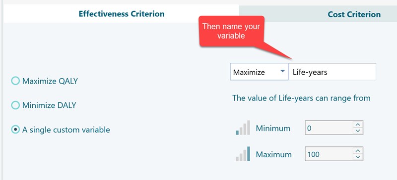
Custom effectiveness variable defined as Life Year for the life expectancy Markov model, including name, symbol, and unit fields.

For this analysis we do not care about cost, only life years, so there is nothing to set for cost. Just click Proceed. The wizard then asks you to set the reward for the "Well" state. Set the life year value to 5, since each cycle in the Well state is worth 5 years of life.

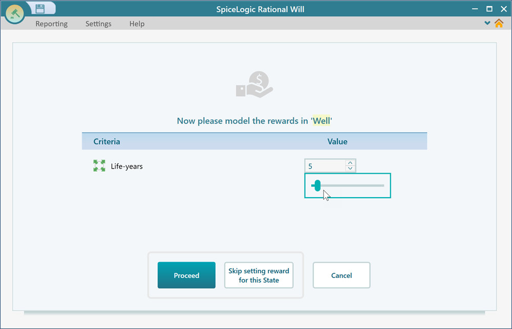
Reward editor for the Well state with the Life Year value set to 5, awarded each cycle the cohort remains in Well.

Now click "Proceed". The wizard asks you to set a reward for the "Dead" state. A dead person gains no life years, so you can either set the value to 0 or click the "Skip getting a reward for this state" button. Either way the result is the same. Once you do this, your finished Markov Model appears as a Decision Tree diagram.

Step 6: Reading the Result

In the diagram, the expected value is shown above the node. Here the expected life year comes out to 76.87. That number is the answer we were after. The life expectancy of this group is 76.87 years. It is the average number of years a person in the group can expect to live, given the age-based death rates you entered.

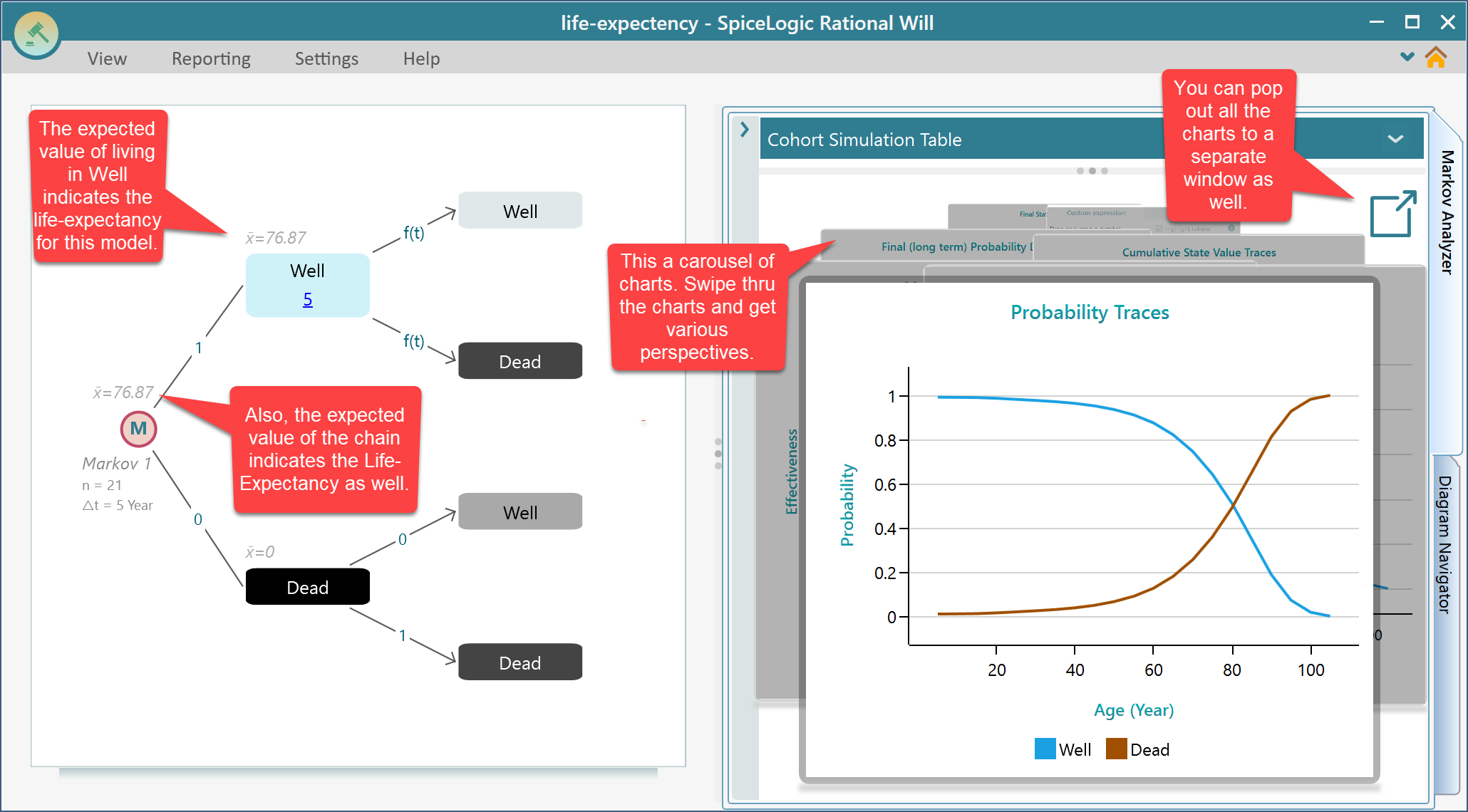
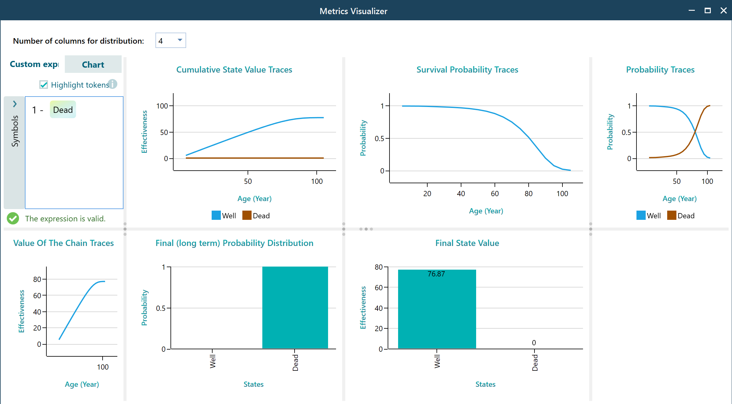
Completed life expectancy Markov model rendered as a decision tree diagram, with the simulation's expected value displayed at the root.

When you click the pop-out button, the charts open in a grid so you can see them all together.

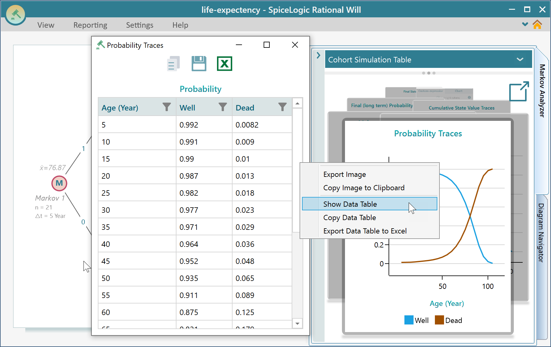
Pop-out window displaying every Markov analyzer chart for the life expectancy run laid out as a single scrollable grid.

To see the numbers behind any chart, right-click on that chart and choose the data table. You can also export that table to Excel if you want to work with the figures somewhere else.

Data table behind a Markov life expectancy chart, exposed via right-click and exportable to Excel for further analysis.

For a clean, organized view of how the group moves through the states over time, use this panel to get the cohort simulation traces. These traces show, cycle by cycle, how many people are left in each state. For example, you can watch the Well count drop and the Dead count climb as the group ages.

Cohort simulation trace table listing, for each cycle, the population in each state across the lifetime of the life expectancy Markov run.

Step 7: Modifying and Refining the Model

Once you finish the step-by-step wizard, the Decision Tree opens showing your Markov Process diagram. From here you are free to change anything: the states, the transition probabilities, the rewards, or all of them. This is handy when you want to test a what-if, such as a lower death rate, without building the model again from scratch. To learn how to edit the model directly on the diagram, see this page.

Calculating Life Expectancy with time variant probabilities