


Monte Carlo Simulation
Real life is full of uncertainty. That does not mean you have to leave everything to chance. There is a way to put numbers on uncertainty, and that is exactly what Monte Carlo Simulation does. Before we get into it, let's start with the idea of a Random Variable.
What is a Random Variable?
You already know this:
Profit = Revenue - Expense
Looking back at last year is easy. You know your revenue and you know your expense. You plug both numbers into the formula and you get a profit figure. One known number out, two known numbers in.
Predicting next year is a different story. You do not know what your revenue or your expense will be, so you cannot just calculate a single profit figure.
You might try to list out the possibilities by hand, like this:
If Revenue is $100 and Expense is $20, Profit is $80.
If Revenue is $200 and Expense is $30, Profit is $170.
.........
The trouble is there is no end to it. Revenue and expense can each take on endless values, so the number of combinations is endless too. You cannot do that by hand.
Here is the better way. Based on your experience and your past records, you can usually describe revenue and expense as probability distributions instead of single guesses. Once you do that, you can work out profit as a probability distribution too.
So the formula turns into this:
Probability Distribution of Profit = Probability Distribution of Revenue - Probability Distribution of Expense
That raises a fair question. How do you subtract one probability distribution from another? A distribution is not a single number you can type into a calculator and hit the minus button.
The answer is Monte Carlo Simulation. It lets you treat Profit as a random variable when Revenue and Expense are random variables.
Monte Carlo Simulation works by taking many random samples. So let's be clear about what random sampling really means.
Random Sampling
Picture this probability wheel, like a roulette wheel.

If you spin this wheel and let it stop, what would you expect on average, red or blue? Out of every 4 spins, you would expect about 3 reds and 1 blue. That is because red covers 75% of the wheel and blue covers 25%. In other words, the result follows a probability distribution: red is 0.75 and blue is 0.25. Random sampling is just that idea put to work. You build a wheel that matches a probability distribution, then spin it to draw a sample.
For example, say you have a probability distribution like this:
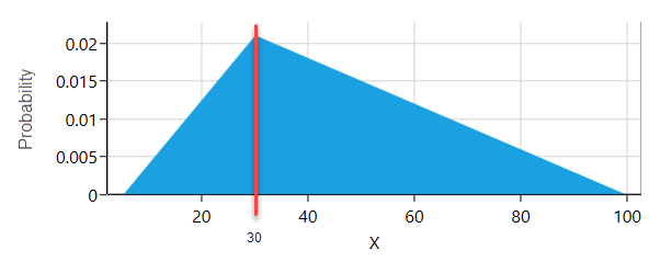
To draw a random sample from this distribution, you build a wheel where every possible outcome gets its own slice. The size of each slice matches that outcome's probability. Look at the triangular distribution above. The value 30 has a probability of 0.02. So on the wheel there is a slice for the value 30, and it takes up 2% of the wheel. Spin that wheel and stop it 100 times, and you would expect the slice for 30 to come up about twice. Every probability distribution has a math formula for this kind of wheel. Most of those formulas are messy to work out by hand. The good news is that when you use the SpiceLogic Rational Will or Decision Tree Software, the software does all of that math for you, so you can stay focused on the decision itself.
How Monte Carlo Simulation evaluates a function of random variables
So far you know what a random variable is and what random sampling is. Now suppose you are the project manager on a new project, and you need to predict the profit. From your past data, you have worked out a probability distribution for both Revenue and Cost.
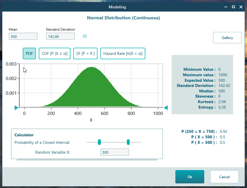
Say your Revenue follows a Normal Distribution, shown below.
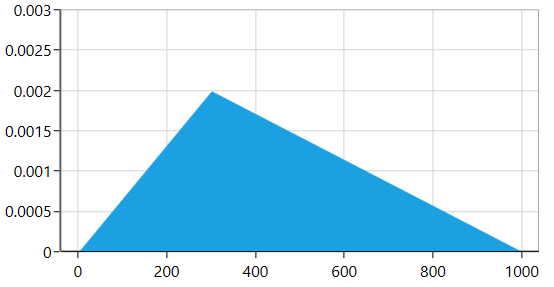
And your Expense follows a Triangular Distribution, shown below.
As we said earlier, you could try to write out endless combinations like:
Combination 1: Revenue $500, Expense $300
Combination 2: Revenue $501, Expense $301
….
.....
You would be buried in no time. There is no practical way to list them all by hand.
This is where Monte Carlo Simulation steps in. The idea is simple. Draw one random sample from the Revenue distribution. Say you get $500. Then draw one random sample from the Expense distribution. Say you get $200. So for this first round, profit is $500 - $200 = $300.
Now draw again. Say this time Revenue is $400 and Expense is $300. So for the second round, profit is $100.
Keep repeating, usually 10,000 times or more.
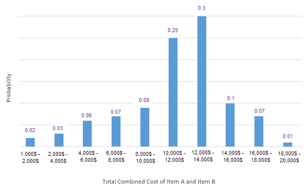
After thousands of samples, you can sort the results into a histogram. The X-axis shows ranges of profit, and the Y-axis shows how many of your random samples landed in each range.
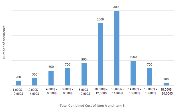
From the chart above, you can read off that out of 10,000 samples, 200 landed in the profit range of $1,000 to $2,000, 300 landed in the $2,000 to $4,000 range, and so on.
Since you have a count for each range, you can turn each count into a probability. Just divide the sample count in a range by the total number of samples (10,000).
So the probability of the $1,000 to $2,000 range is 200 / 10,000 = 0.02. Do that for every range and you end up with the probability distribution of profit, like this:
This method of finding the probability distribution of a dependent random variable is what we call Monte Carlo Simulation.
Step by Step Modeling Example
Let's model the function we have been talking about, Profit = Revenue - Expense, where both Revenue and Expense are random variables.
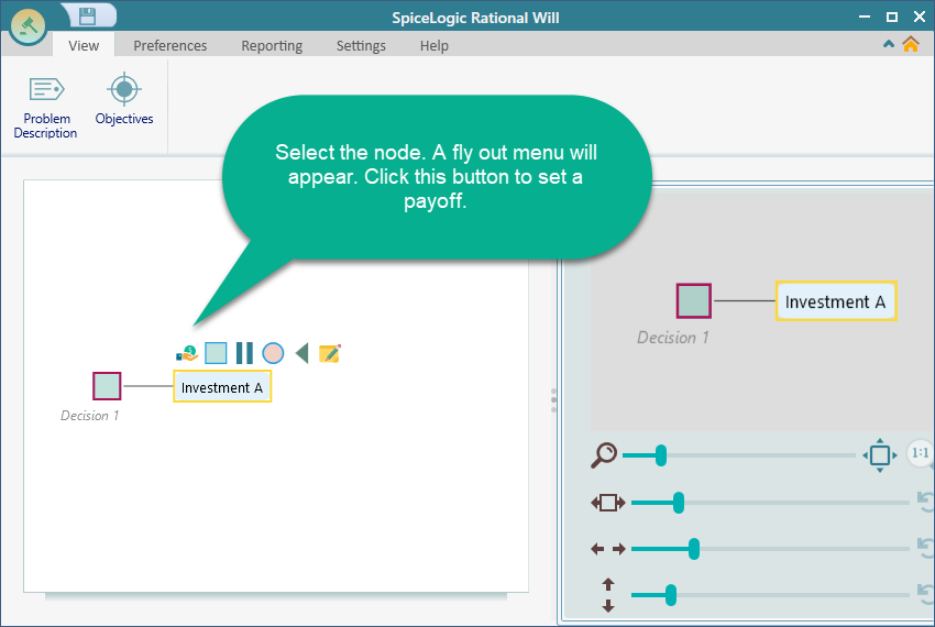
Start the Decision Tree Analyzer and build a simple tree like the one below, with just one Decision Node and one action.
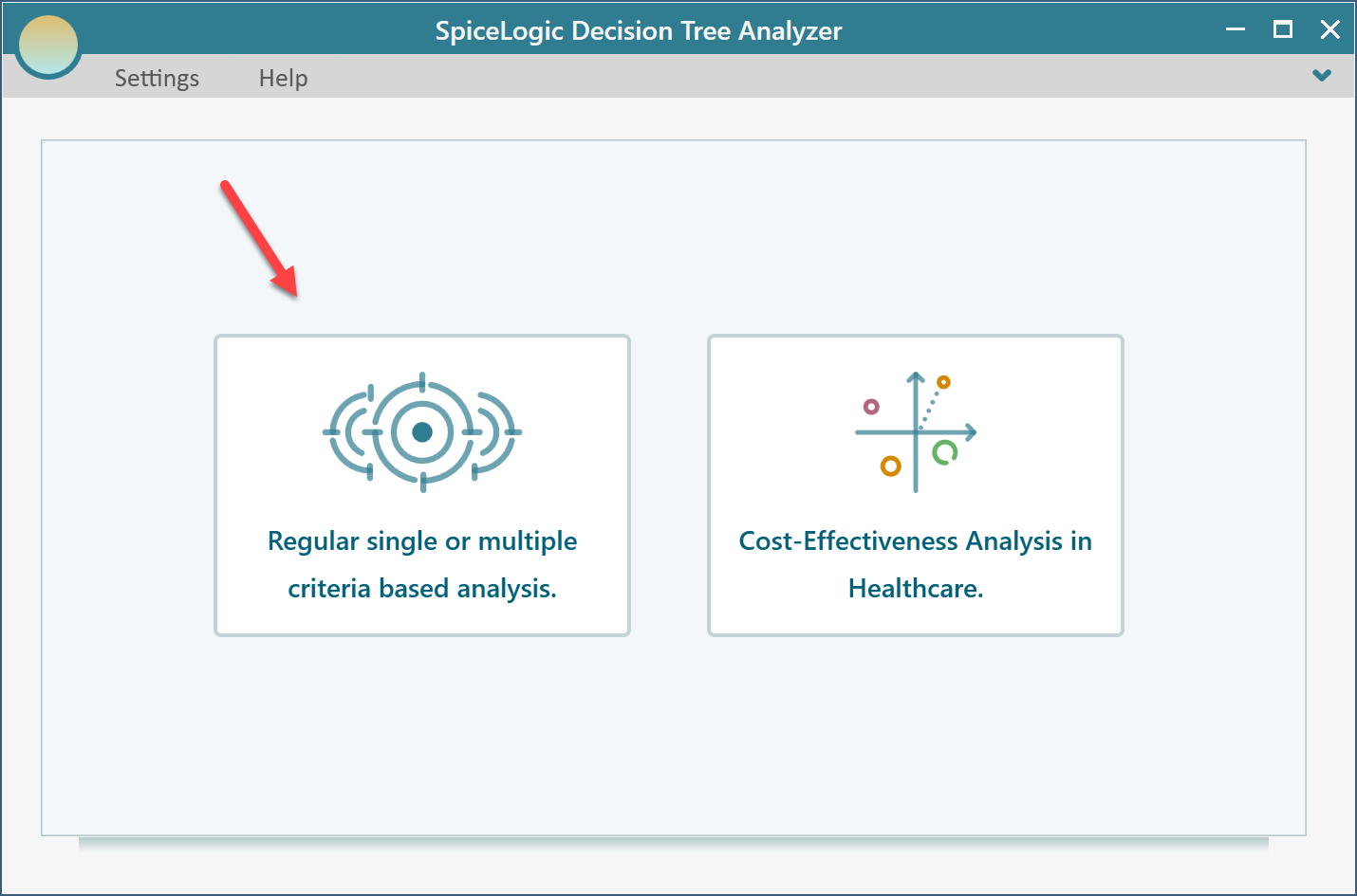
The first time you click the "Pay off" button in a project, the software asks whether you want a regular single or multiple criteria analysis, or a Cost-Effectiveness analysis. Choose the first option.
You will then see the screen below. Select "Maximize" and type in "Revenue", as shown here.

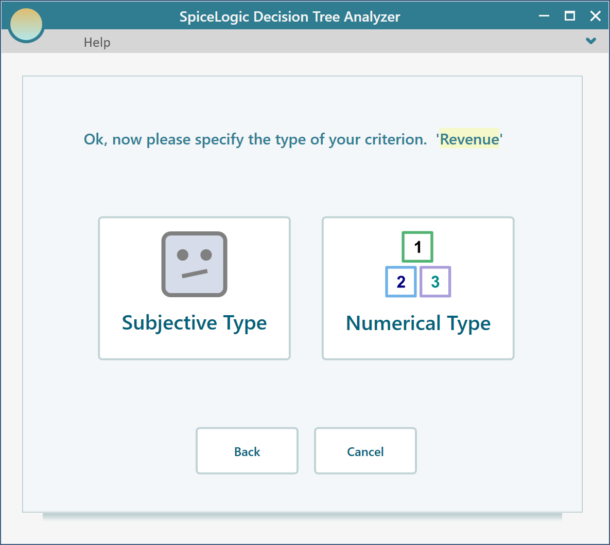
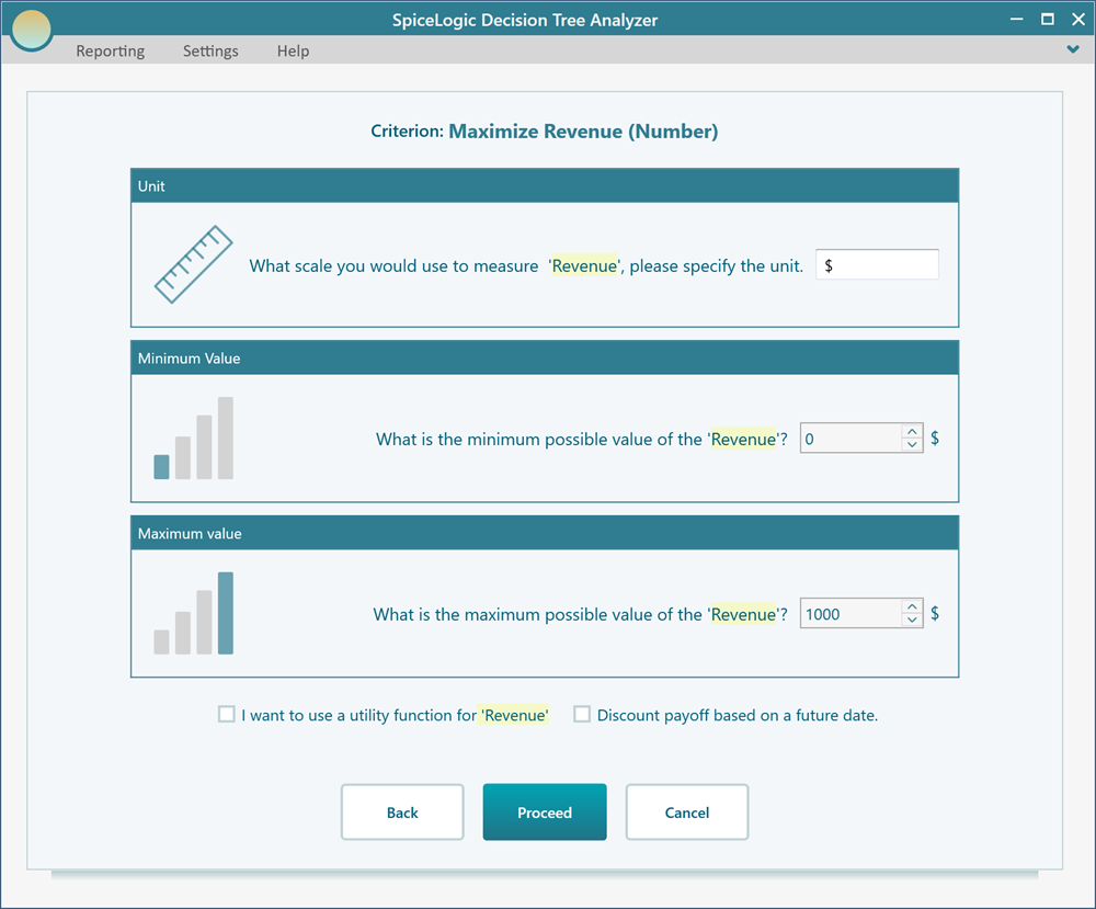
Click the "Proceed" button. The software asks what type of criterion this is. Select "Numerical Type".
Next you are asked for a minimum value, a maximum value, and a unit. Use $ as the unit, 0 as the minimum, and $1000 as the maximum.
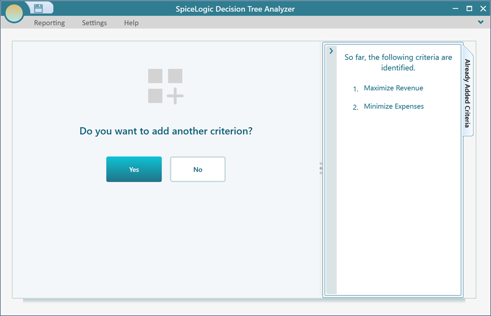
Click "Proceed". The software asks whether you have another criterion to add. Click Yes. Then, in the same way, create a numerical objective called "Minimize Expenses".
When that second criterion is done and you are asked whether to add another, answer "No".
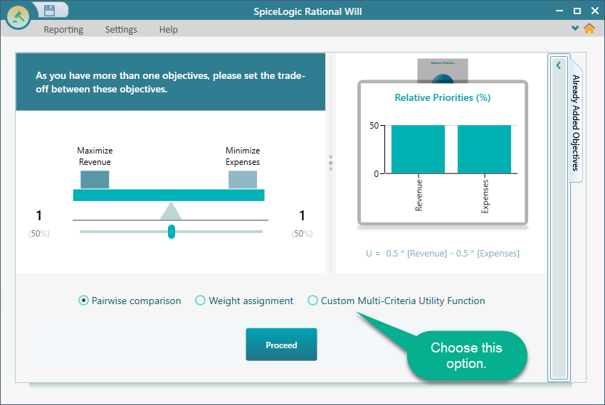
Now you are asked to set up a trade-off between the two criteria. This forms a multi-criteria utility function. You have several choices here, such as pairwise comparison, a custom expression, and more. For this example, choose the Custom Multi-Criteria Utility Function from the screen below.
When you click the Custom Multi-Criteria Utility Function box, a math equation editor opens up. In this editor you can write full math expressions, for example sqrt([Revenue]) - ln([Expenses]). Our expression is much simpler. It is just [Revenue] - [Expenses], so keep it exactly as shown here.
![Custom Multi-Criteria Utility Function editor with the rich math expression [Revenue] - [Expenses] entered to define Profit.](https://spicelogicprodstorage.blob.core.windows.net/documentation/DecisionTreeAnalyzer/category-84/page-321/section-2274/custom-utility-expression-revenue-minus-expenses.png)
Click the "Proceed" button. You are taken back to the decision tree, and the payoff editor appears. Enter simple values for now: Revenue $500 and Expenses $200. The node shows a value of $300, which is correct, since our custom expression gives Revenue - Expenses = 500 - 200 = 300.
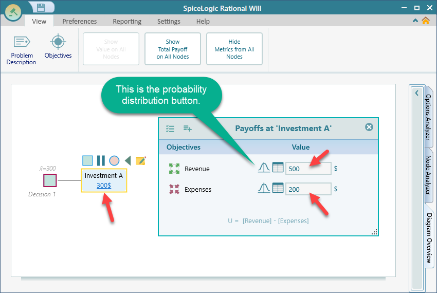
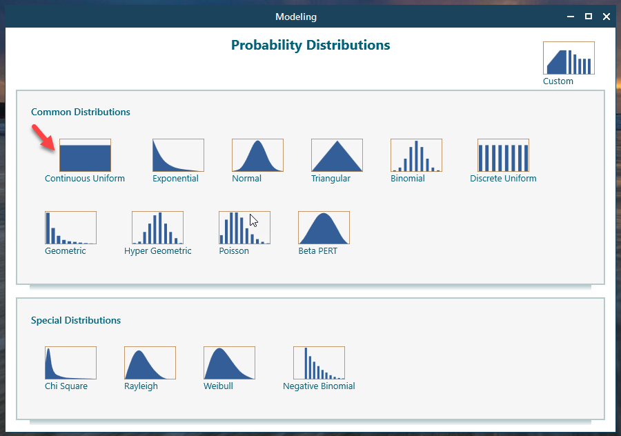
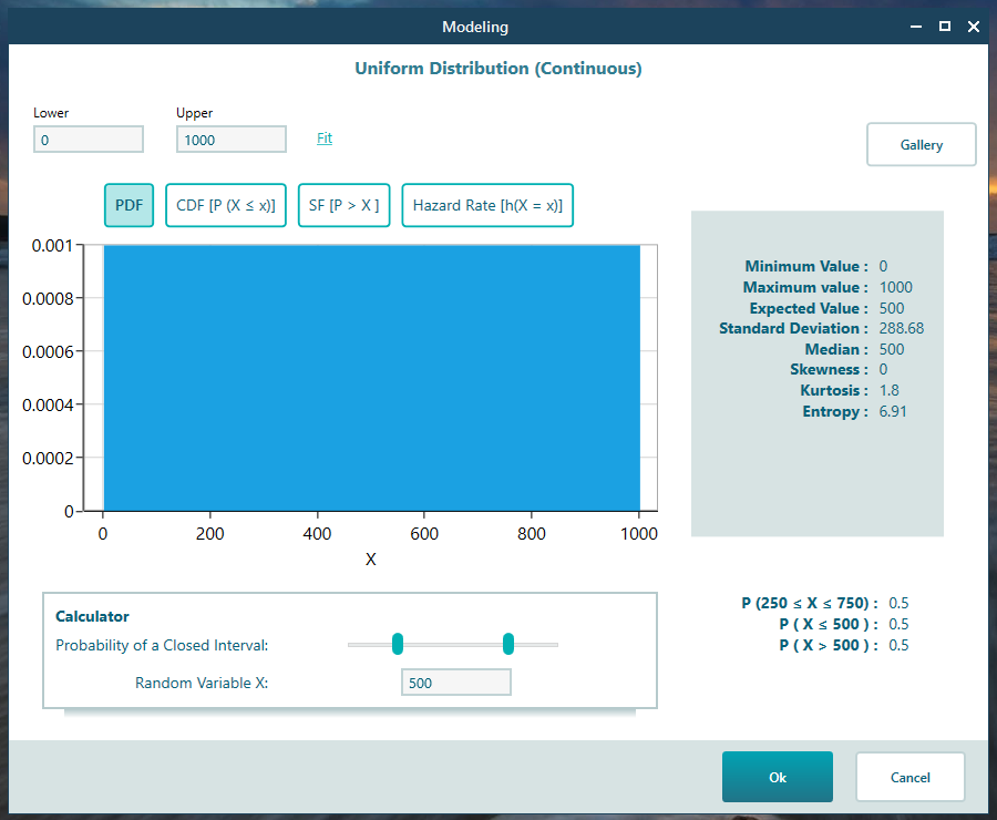
Now let's give Revenue a probability distribution. Click the probability distribution icon in the Revenue row, shown in the screenshot above. The probability distribution window opens. Click the "Continuous Uniform" distribution, shown below.
We left the default settings as they were and clicked OK.
Do the same thing for the Expense criterion. This time, pick the "Exponential" distribution from the gallery. Leave the defaults and click through. The payoff editor in the decision tree will now look like this.
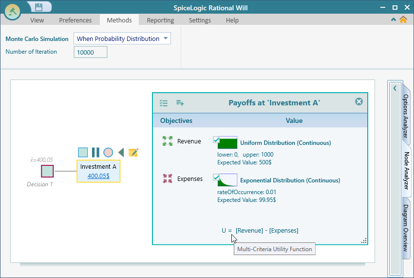
Now for the interesting part. Open the Options Analyzer and look at the Risk Profile chart carousel.
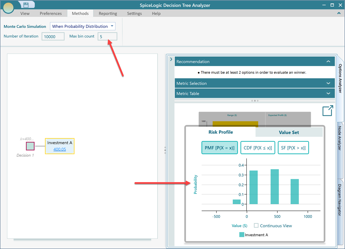
Keep the action node "Investment A" selected in the diagram and expand the "Node Analyzer" tab. In the Ribbon, under "Monte Carlo Simulation", you will find a number box labeled "Number of Iteration". Set it to 10,000. More iterations give a more accurate result.
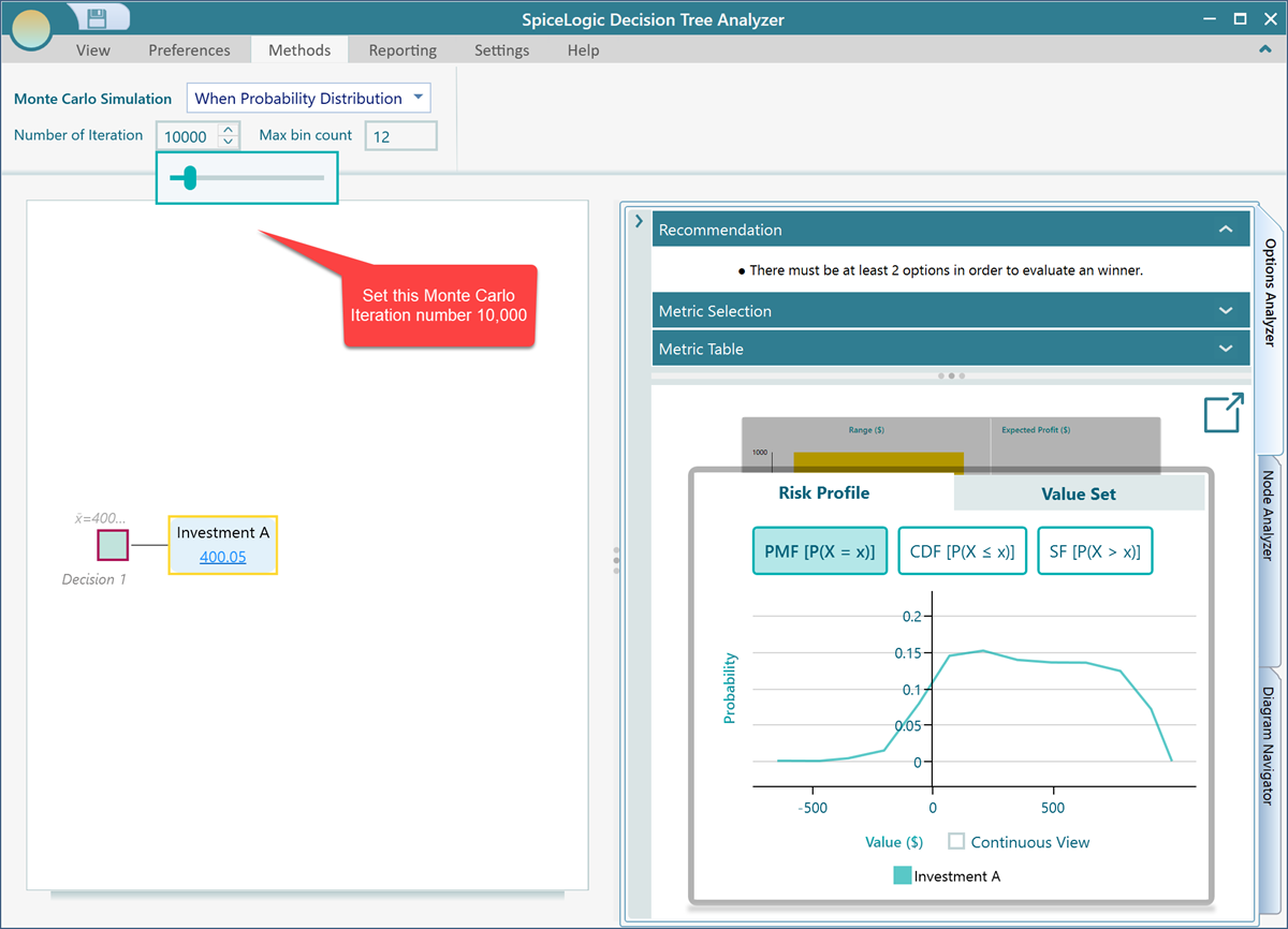
And there it is. You can now see a probability distribution for our random variable "Profit", which equals Revenue minus Expenses. The Decision Tree Analyzer ran a Monte Carlo simulation behind the scenes and produced this distribution. The chart is the result of subtracting one probability distribution from another, exactly as we defined in the custom expression editor.
If you add a second action node to the Decision Node, the software compares them. The action with the higher expected value is the one it recommends as the better choice.
In the ribbon there is another number box called Max bin count. A bin is a segment that the simulation results get sorted into. Use a lot of bins and the results spread out evenly across all of them, which often does not tell you much. Use very few bins and the differences between bins stand out more, which can be more useful for many analyses. By default the software uses 12 bins. Let's change it to 5 and see what happens.
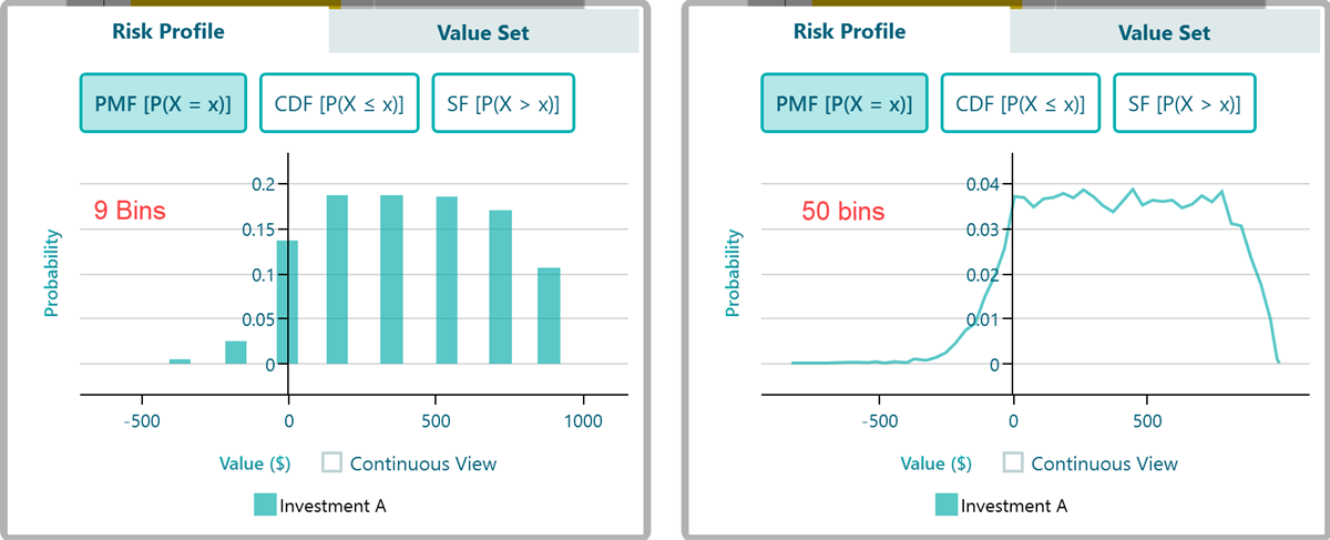
Now the results are grouped into just a few segments. The screenshot below shows the same risk profile with 9 bins and then with 50 bins, so you can compare.
A real random function as a decision tree
Let's model something real. Say you are planning a vacation and you can travel by car or by plane. If you drive, your car might break down on the road, and the repair could cost anywhere within a range. And as you know, plane ticket prices never stay still, they change all the time. Assuming you already know how to create a decision tree in the software, let's build one like this:
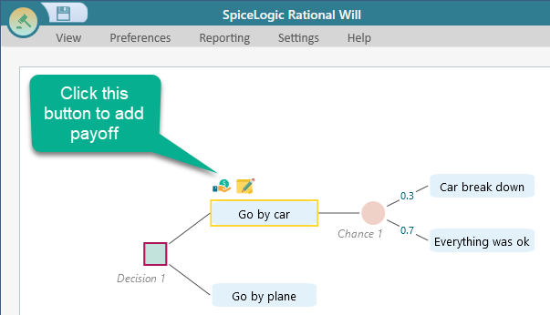
Let's say the chance of the car breaking down is 0.3. Set that probability as shown in the screenshot above.
Now create an objective called "Minimize Cost". From the flyover menu on the "Go by car" node, click the "Payoff" button. The objective wizard opens. Create the "Minimize Cost" objective the same way as before: choose Money type or Number type with the unit "$", a minimum of 0, and a maximum of $1000, as shown below.
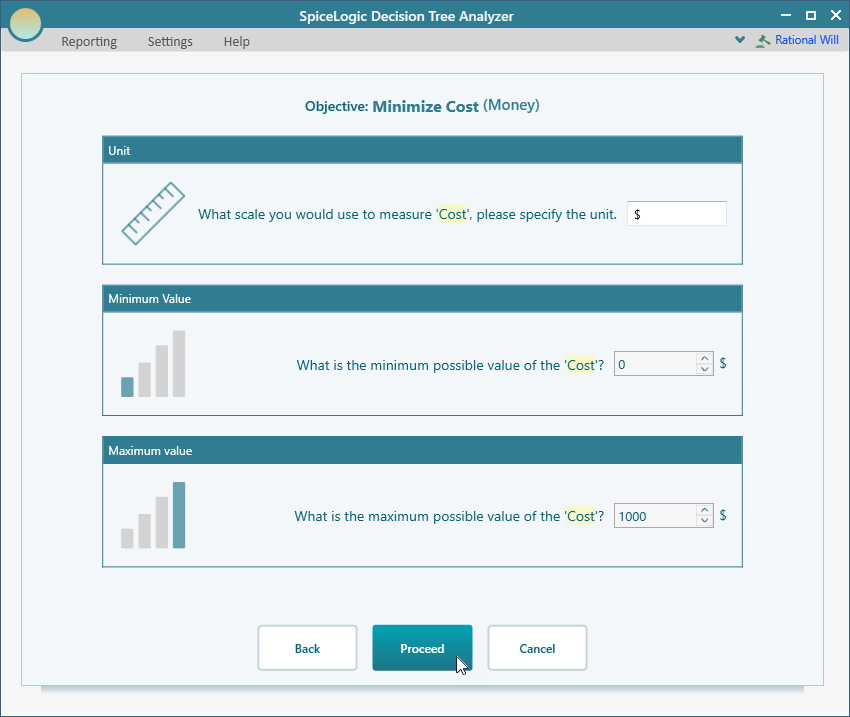
Click Proceed. When you are asked whether there are any more objectives to add, answer "No". You are then taken to the decision tree, like this.
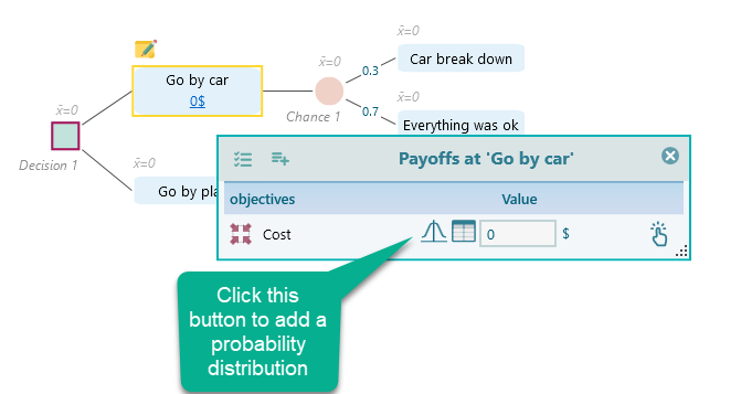
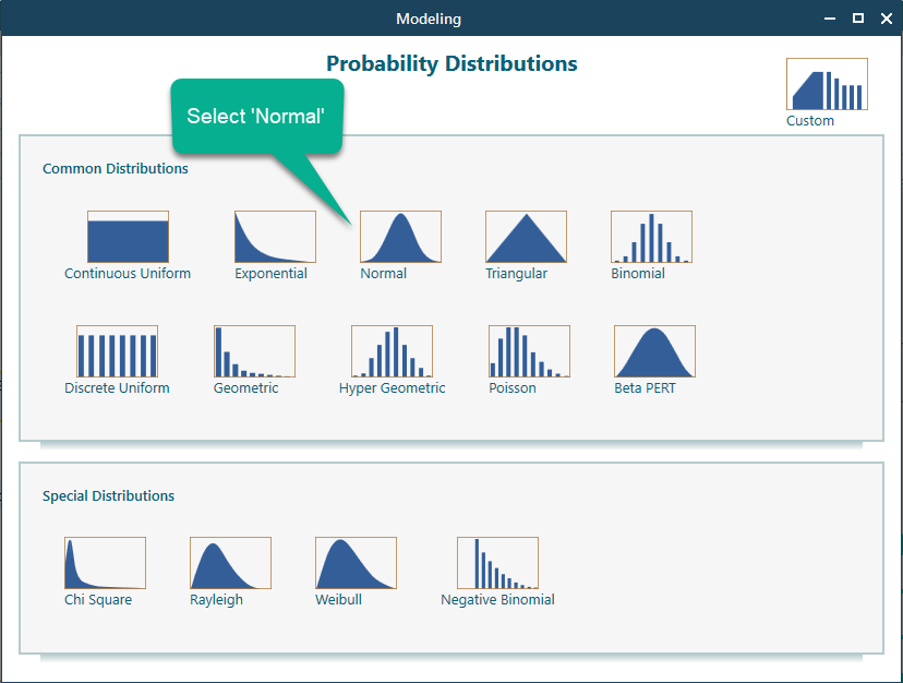
Now think about the cost of driving. It could land anywhere from $100 to $500, because you cannot be sure about gas prices along the way, how much food you will buy, and so on. Still, your best guess is that it will probably come in around $300, with $100 or $500 being less likely. A normal distribution with a mean of $300 fits that picture well. Click the probability button in the payoff editor and choose "Normal Distribution" this time.
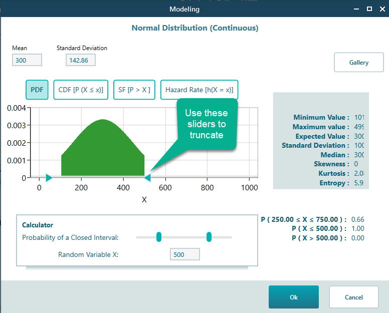
Once you pick the normal distribution, you can set the mean and the standard deviation.
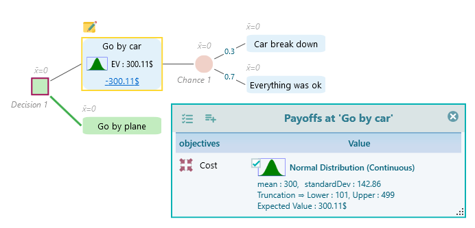
Click OK to accept the distribution you set up. The decision tree will now look like this.
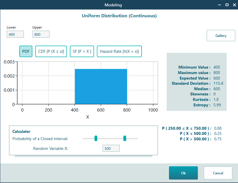
Now set a probability distribution for the car breakdown cost. You figure it could be somewhere between $400 and $800, but you have no idea which value is most likely. So a uniform distribution is a good fit. This follows the principle of indifference: if you have no reason to believe one outcome is more likely than another, you treat them all as equally likely. Since you cannot guess what kind of breakdown might happen, give every value in the range the same chance with a continuous uniform distribution. Just like the driving cost, attach a uniform distribution that runs from 400 to 800, like this:
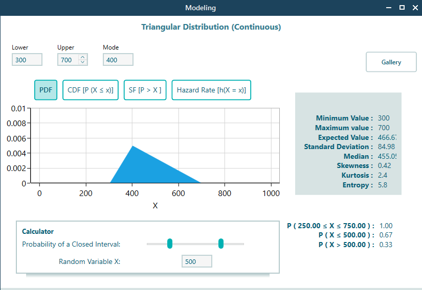
Now set a distribution for the plane cost. Your best guess for the most likely price is $400, but it could be higher or lower, perhaps anywhere from $300 to $700. You could use a triangular distribution or a normal distribution, whichever you feel more confident about. A triangular distribution makes good sense here, like this:
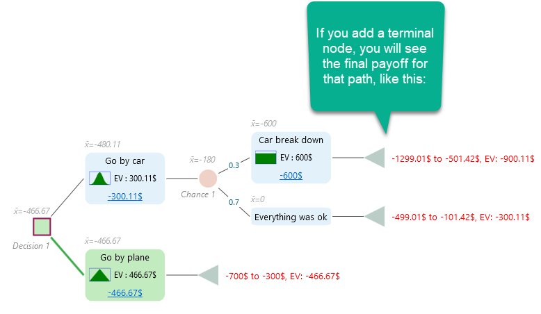
With all of that in place, the decision tree will look like this.
The modeling is done. Now expand the Options Analyzer panel to see all the calculated results. And here is the nice part: the Monte Carlo simulation has already run for you. Look at the probability distribution in the Risk Profile panel. That distribution is the output of the Monte Carlo simulation.
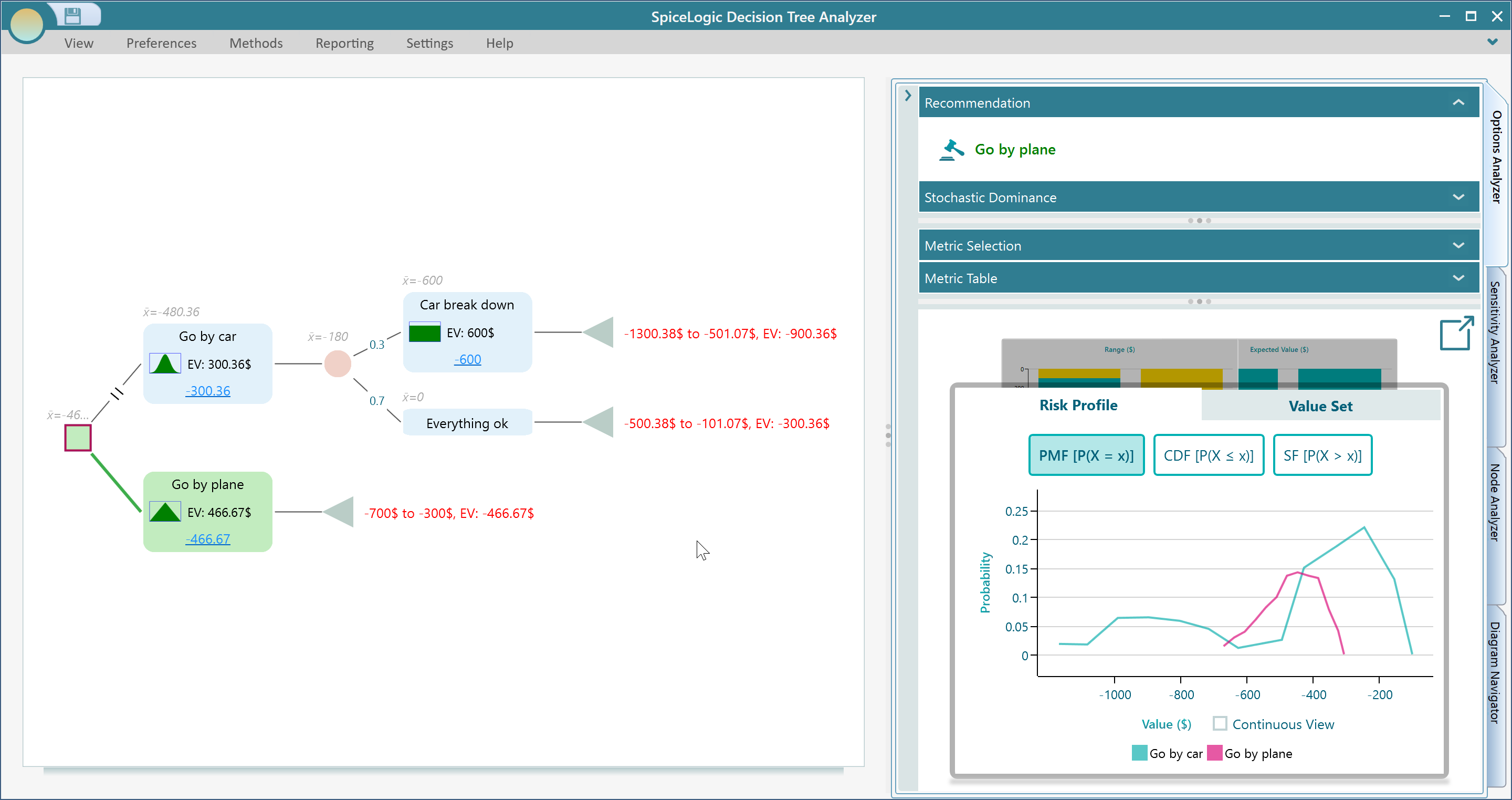
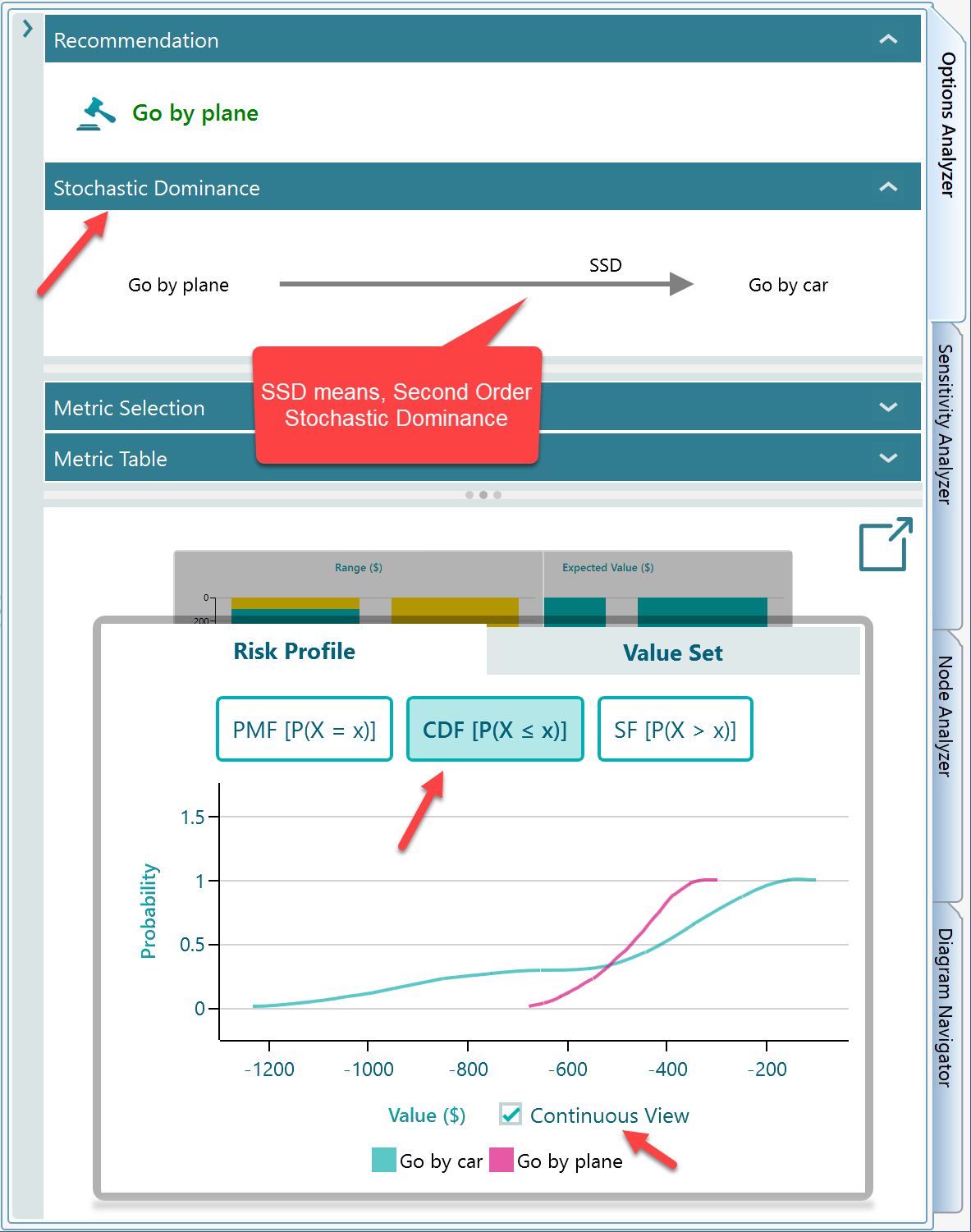
You can resize the panels for a clearer view, as shown below. Notice that Stochastic Dominance is also worked out from the risk profile. Expand the Stochastic Dominance panel to see the dominance diagram.
In the Risk Profile chart, switch to the CDF view to see the Cumulative Distribution Function, which is a clearer way to read stochastic dominance. Also tick the Continuous View checkbox, shown in the screenshot below, for a smoother graph.
How the result was calculated
So the SpiceLogic Rational Will or Decision Tree Software produced the probability distribution in the Risk Profile panel. But how? It built thousands of random samples, like this:
1. It drew a random sample from the cost distribution on the "Go by car" node. Call that value "p". Then, using the probability wheel, it picked an outcome at the chance node based on the event probabilities (0.3 for the car breaking down). If the "Car breaks down" branch came up on the wheel, the software drew a random sample from the breakdown cost distribution. Call that value "q".
So in the first round, the total cost is "p + q".
2. It repeated this process thousands of times, producing a large set of outcomes. The software then chose to show the results in up to 100 groups. It works out a group width so the outcomes fall into at most 100 groups. In the screenshot above, the tooltip shows the group "-932.36 to -920.36", and the probability of landing in that group is 0.01.
Options for Monte Carlo Simulation
By default, Monte Carlo Simulation is turned on automatically whenever a probability distribution is used.
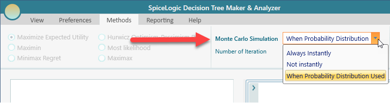
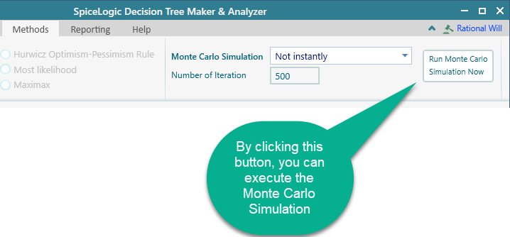
You can turn that automatic behavior off by changing the drop-down to "Not Instantly", as shown in the screenshot above. With "Not Instantly" selected, you get a button to run the Monte Carlo simulation by hand, so you can run it whenever you want.
If you set the option to "Always Instantly", then Monte Carlo simulation runs whenever there is at least one chance node in the tree, whether or not any probability distribution is used, and it generates the Risk Profile.