Markov Models in a Decision Tree: Chains and MDPs

SpiceLogic Decision Tree Software lets you build a Markov Chain or a Markov Decision Process with a special node called the Markov Chance Node. You can attach a reward (or payoff) to a Markov State or a Markov Action, then run a Utility Analysis or a Cost-Effectiveness Analysis on the chain or the process.

A Markov model fits well when the thing you are studying moves back and forth between a small set of conditions over time. Picture a patient who can be Healthy, Sick, or Dead, and who shifts between those conditions year after year. A plain decision tree has trouble with this, because a tree only moves forward and never loops back. A Markov model handles the looping with no fuss. The patient can get Sick, recover to Healthy, and get Sick again, and the model tracks all of it.

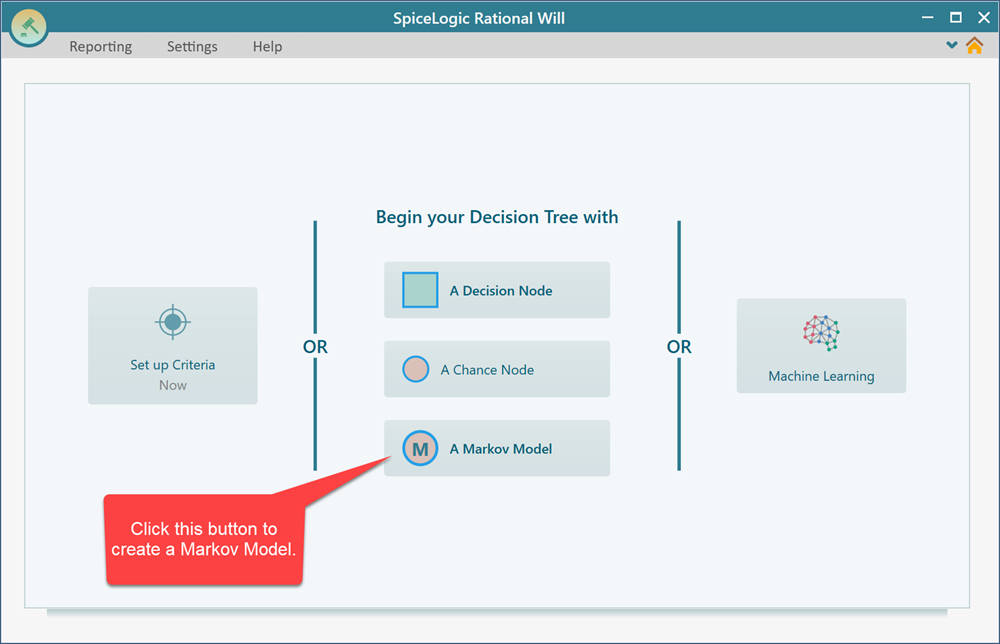
Just like a Decision Node or a Chance Node, you can use a Markov Chance Node as the root of your model. You will find this option right on the software start screen. When you open the Decision Tree software, look for the button labeled "A Markov Model". Click it, and you get a decision tree whose root node is a Markov Chance Node. Before the diagram opens, a step by step wizard appears. It walks you through the basics: what your Markov States are, the odds of moving between them, and so on. When you finish, the wizard builds the Markov diagram for you.

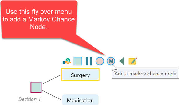
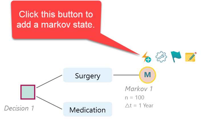
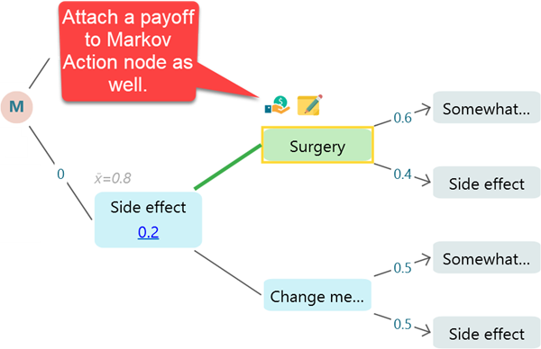
Decision Tree Analyzer start screen with the Markov Model option highlighted to use a Markov Chance node as the root of a new decision tree.

You do not have to start from scratch with a Markov model. If you already built a decision tree, you can attach a Markov model to an action node, as shown in the screenshot below. This is handy when one branch of your decision plays out over many cycles while the rest of the tree is a normal one-time choice. For example, your tree might first ask whether to run a screening program at all. The "do nothing" branch is a single outcome, but the "screen everyone" branch leads into a Markov model that follows the group year by year. You can keep both styles in the same tree.

Fly-over toolbar on a decision tree action node showing the Markov Chance node button used to attach a Markov model to an existing action.

The wizard for building a Markov model

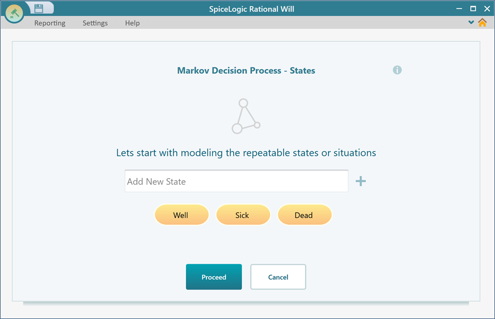
As soon as you click the Markov Chance node button, or the "A Markov Model" button, a wizard opens and helps you build the model one step at a time.

A Markov Chain or a Markov Decision Process is made of Markov States. A Markov State is a lot like a Chance node in a decision tree, with one key difference: a Markov State can be cyclic. That means a state can move to another state and later come back to itself. For example, a Sick patient can recover to Healthy, then fall Sick again. A normal tree cannot do that, but a Markov State can.

From this first screen you add as many states as your model needs, then move on to the next step. If you are modeling a patient, you might add Healthy, Sick, and Dead here. If you are modeling a machine, you might add Running, Degraded, and Broken. Name them in plain words so the rest of the model is easy to read.

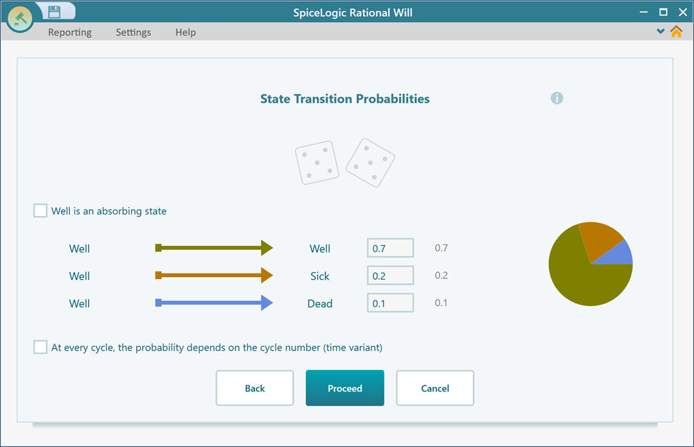
First step of the Markov Model wizard in Decision Tree Analyzer where the user adds named Markov states (such as Healthy, Sick, Dead) to the chain.

From there, the wizard keeps asking you for the pieces it needs: the transition probabilities between states, any actions you want to add, the criteria or cost-effectiveness parameters you care about, and finally the utility values or the cost and effectiveness values for each state or action. The screenshot below shows the step where you set the transition probabilities for a state. You enter the odds of leaving that state for each of the others in one cycle. The wizard takes one state at a time, so you only think about one row of numbers at a time instead of the whole grid at once.

Wizard step for entering the transition probabilities from a Markov state to every other state, with input boxes for each destination probability.

The wizard is easy to follow. Go through it once and you will not get lost. When you finish, the model is created and you see a diagram that looks much like a decision tree.

The wizard is optional. If you would rather build everything by hand, click Cancel and you go straight to the diagram, where you can add states, set transition probabilities, and adjust anything yourself. The next section shows how to change a Markov model that the wizard already built. The same steps apply if you skip the wizard and do it all by hand, so it is worth reading either way.

Creating a Markov State from the diagram

Once you have a Markov Chance node on the diagram, you add states the same way you add children to a regular chance node. Each child you add becomes a Markov State. So if you want three states, you add three children, and each one shows up on the diagram ready to be named and wired into the rest of the model.

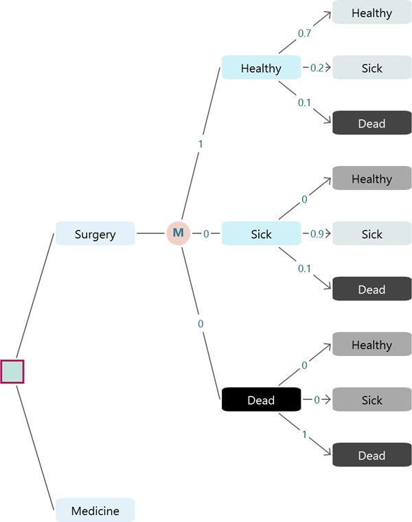
Fly-over toolbar on a Markov chance node (labelled Markov 1, n = 100) with the Add Markov State lightning-plus button highlighted by a callout.

Say you add three states under a Markov Chance node and name them "Healthy", "Sick", and "Dead". You will see that all of the states get connected to each other, which is what completes the transition system. Every state can, in principle, lead to every other state, so the software wires them up for you and lets you fill in the probabilities later. You do not have to draw a single arrow by hand. If a move should never happen, like Dead going back to Healthy, you handle that later by setting that transition probability to 0.

Generated Markov process diagram in Decision Tree Analyzer with Healthy, Sick, and Dead states fully connected by transition arrows.

Opening the Markov settings from the diagram

It is a good idea to review and set up your Markov simulation settings before you run the simulation or start filling in transition probabilities. To solve the chain or the process, the software runs a cohort simulation. That means it follows a large imaginary group of subjects through the states cycle by cycle and tracks where they end up. Setting the simulation up first saves you from rerunning the model later just because a basic setting like the number of cycles was off.

To open the cohort simulation settings, click the fly-over menu icon on the Markov Chance node.

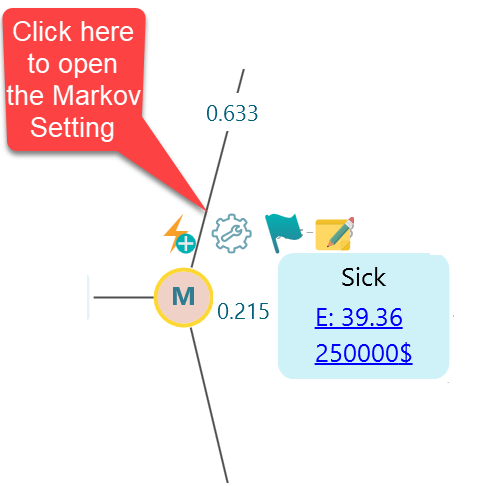
Fly-over menu on the Markov Chance node with the Markov Cohort Simulation Settings button highlighted, opening the simulation configuration for that chain.

When you click that icon, the Markov Cohort Simulation settings for that chance node open up, as shown below. There are a handful of settings here, and they each change the run in a different way, so let's go through them one at a time.

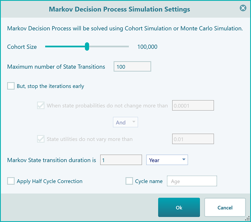
Markov Decision Process Simulation Settings dialog with cohort size 100,000, maximum number of state transitions 100, transition duration 1 Year, optional cycle name, and Apply Half Cycle Correction checkbox.

There are several things you can set here to shape your simulation results.

Cohort Size: This is the size of the imaginary group the software runs through the model. The default is 100,000, which is plenty for almost any scenario, so most of the time you can leave it alone. If you want a slightly smoother result, you can raise it and watch the numbers settle a little more.

Maximum number of state transitions: This is how many cycles the simulation runs. The default is 100, which is fine for most models. For healthcare work you usually set it to match the time span you care about. If you want to study a treatment over the next 10 years and each cycle is one year, set this to 10.

Convergence setting: This tells the program it can stop early once things stop changing. You can have it watch the state probabilities, or the state utility values, or both, and stop the run when they no longer move in a meaningful way. The screenshot above shows the options. This saves time on long runs, since there is no point in grinding through more cycles once the answer has settled.

State transition duration: This is how much real time one cycle stands for, and it matters for two reasons. First, it drives discounting of future values. If your cycles are 5 years apart, the utility a cycle earns gets discounted based on how far in the future it falls. Second, it keeps your probabilities honest. If your transition probabilities were measured assuming each cycle is 5 years, you must set the duration to 5 years so the math lines up. The value you set here also shows up in the charts, tables, and reports.

Half-cycle correction: The "Apply half-cycle correction" checkbox handles a small timing adjustment. In healthcare analysis people often apply it, especially when each cycle covers a long stretch of time, because transitions really happen throughout a cycle rather than all at the end. If you are not sure, leave it unchecked. Most everyday models do not need it.

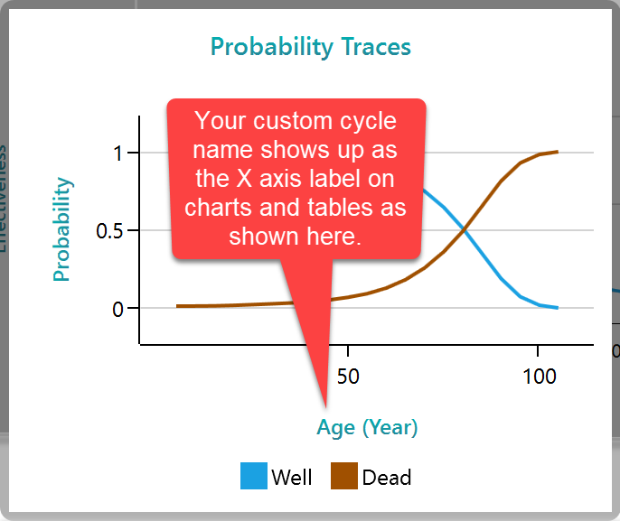
Custom cycle name: If you are studying the life expectancy of a group, your transition probabilities depend on the group's age. In that case, seeing "Age" along the X-axis of your charts and tables is far more useful than seeing a bare cycle number. Check this box to give your cycle number a friendly name. The program already suggests "Age", since that is the common choice for healthcare work. The screenshot below shows how the custom cycle name appears, so you can see why you might want one.

Probability Traces chart showing the custom cycle name (Age (Year)) used as the X-axis label, demonstrating how the user-supplied cycle name flows into Markov charts and tables.

Setting the initial probabilities from the diagram

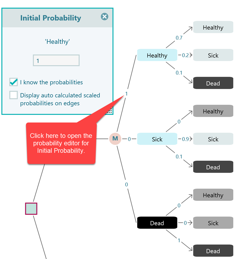
Every Markov chain or process needs a starting point, which means you have to say how likely each state is at the very beginning. These are the initial probabilities. For example, with the states "Healthy", "Sick", and "Dead", you might say the group starts with a 20% chance of being Healthy, a 50% chance of being Sick, and a 30% chance of being Dead. The three numbers add up to 100%, because everyone has to start somewhere.

In practice, models often start everyone in a single state. When that is true, the initial probability of that one state is 1 and every other state is 0. For instance, you might decide everyone begins Healthy.

To set the initial probability of a state, click the probability number, or the '?' shown on the edge, as pointed out here.

Setting the initial state from the diagram

There is a quick shortcut for the common case where everyone starts in one state. Select the Markov State, right-click to open the context menu, and choose the option to set it as the initial state. This sets that state's initial probability to 1 and every other state's initial probability to 0 in a single click, so you do not have to enter them by hand. It is the fast way to say "everyone begins Healthy" without touching three separate numbers.

Right-click context menu on a Markov state with the Set as Initial State command highlighted, which forces that state's initial probability to 1.

Setting the transition probabilities from the diagram

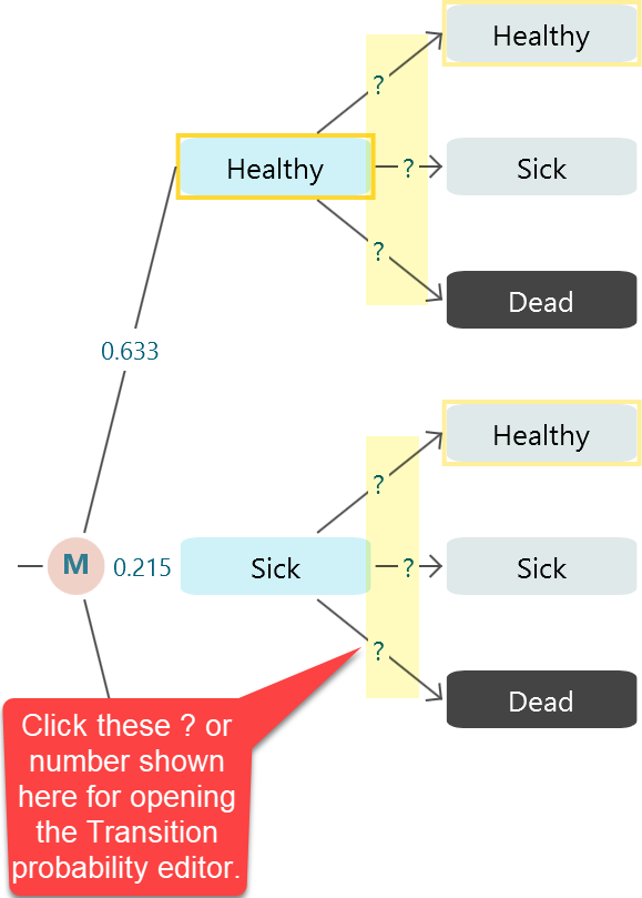
In a Markov chain or process, the states are joined together by transition probabilities, which are the odds of moving from one state to another in a single cycle. Setting them works almost the same as setting the probability of an event on a regular chance node. Once the system is laid out like a tree, as shown below, click the highlighted numbers, or the '?', to set a transition probability. For example, you might say a Sick patient has a 60% chance of staying Sick, a 30% chance of recovering to Healthy, and a 10% chance of moving to Dead in one cycle.

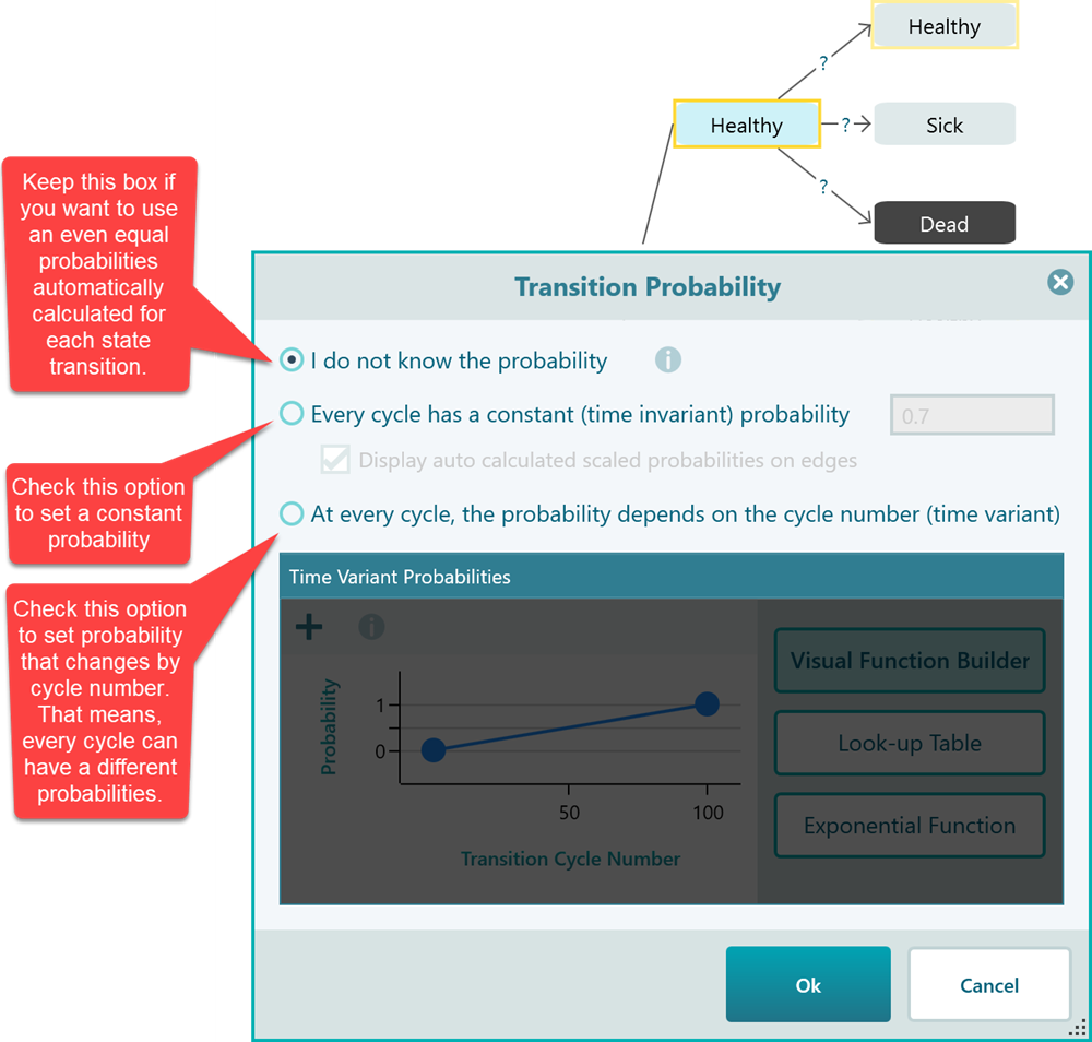
Markov diagram with yellow question-mark placeholders on the transition edges from Healthy and Sick states, and a callout instructing the user to click a question mark or number to open the Transition probability editor.

When you click there, the transition probability editor opens, like this. You type the value for that move, and the editor keeps the rest of the row in view so it is easy to see that the numbers leaving a state add up correctly.

Transition Probability editor offering three modes: I do not know the probability, a constant (time-invariant) probability, or a time-variant probability that depends on the cycle number, with Visual Function Builder, Look-up Table, and Exponential Function options.

Time-variant probabilities

SpiceLogic Decision Tree software lets you define a probability as a function, so the value can change from one cycle to the next instead of staying fixed. This is especially handy for healthcare models, where the odds of a bad event are not the same at every age. A patient's chance of having a stroke or dying climbs as they get older, so a single constant number would not be realistic. A time-variant probability lets the value rise (or fall) over the cycles.

Check the last box to use a time-variant probability, and a set of options for building that function appears.

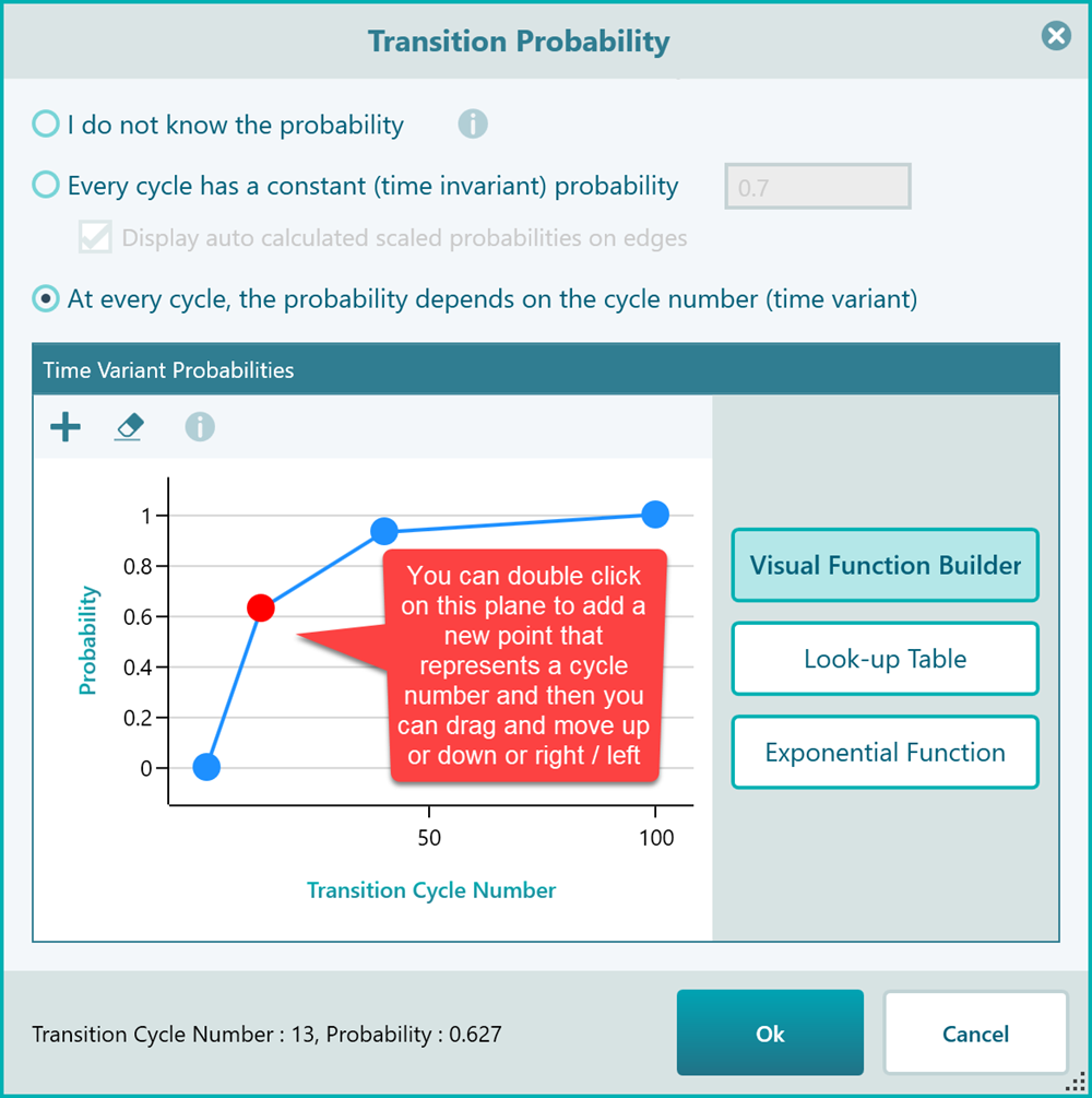
Visual function builder for time-variant Markov transition probability, with a draggable curve plotted against cycle number for points the user adds by double-clicking.

The visual function builder is an easy way to shape a time-variant probability. Double-click anywhere to add a new point, then drag points with your mouse to move them up, down, left, or right until the curve matches what you want. To remove a point, select it and press the DELETE key. So if a risk should stay flat for a while and then climb later in life, you can draw exactly that shape by hand. The next option is a look-up table, shown in the screenshot below.

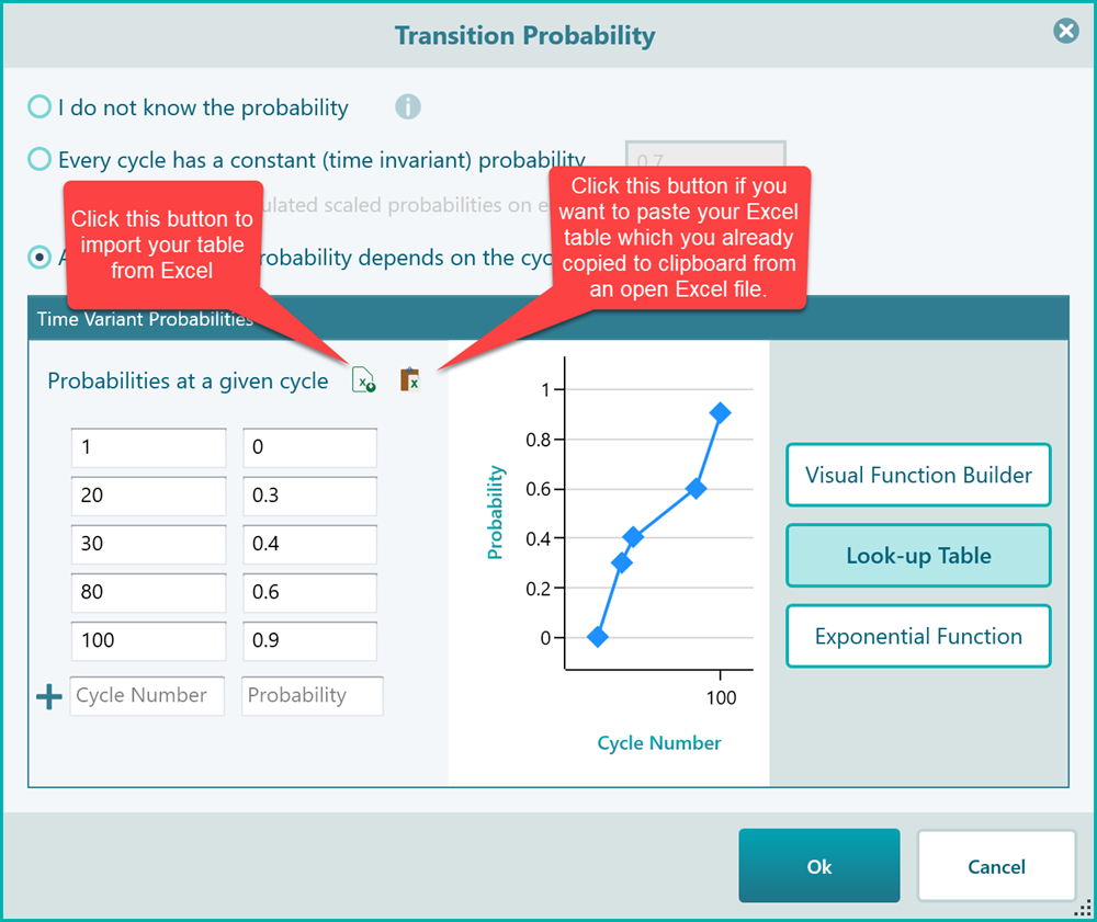
Look-up table option for time-variant Markov transition probability, mapping cycle numbers to probability values with interpolation between rows.

You do not have to fill in a row for every cycle number. Enter the values you know, and the software fills in the gaps by interpolating between the entries you gave it. For example, you might enter a risk at age 50 and again at age 60, and the software works out the in-between years for you.

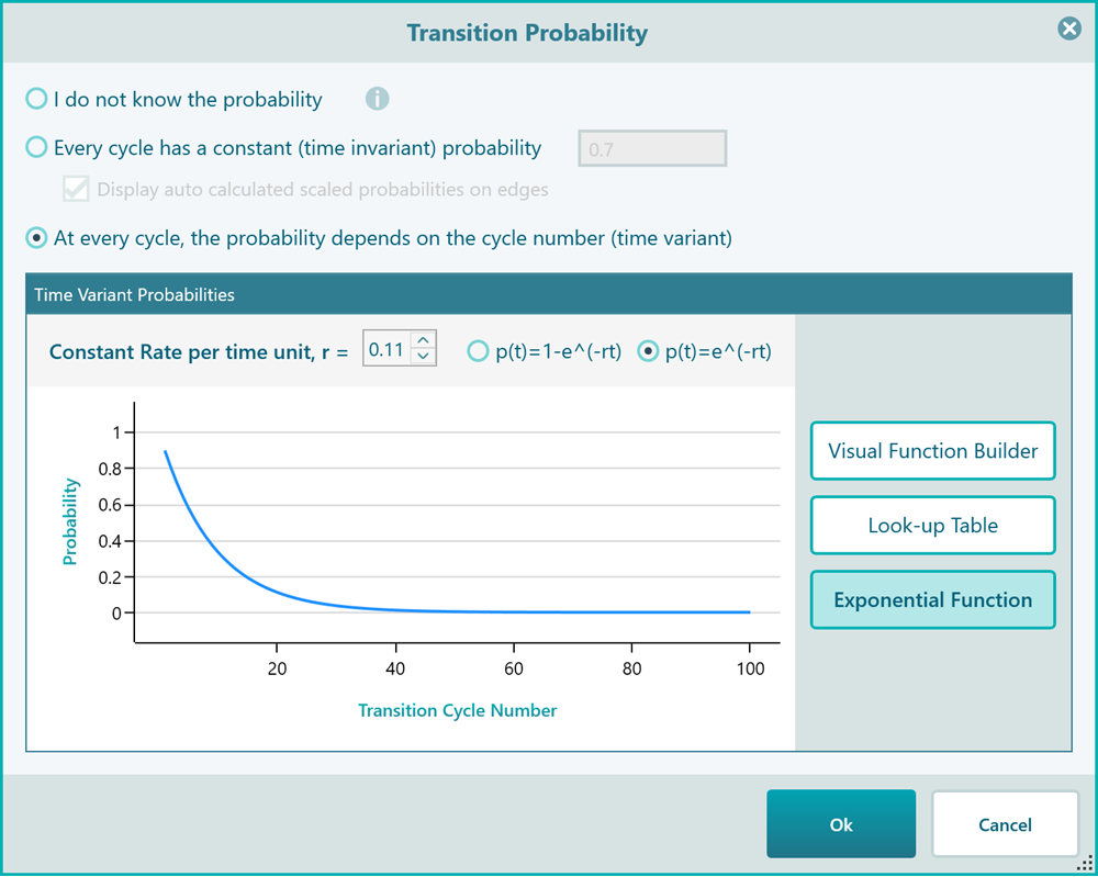
Finally, if your probability changes at a steady rate, you can use an exponential function, as shown below.

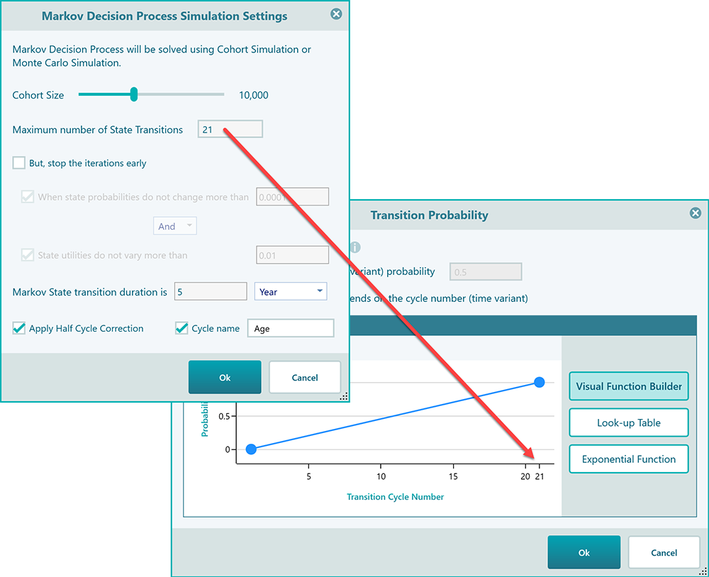
Exponential function option for time-variant Markov transition probability, used when the probability changes at a constant rate per cycle.

You might wonder why the charts and table inputs run up to 100 on the X-axis. That 100 comes straight from your Markov settings, where you set the maximum number of state transitions. Change that number to 21, for example, and the charts and tables in the time-variant probability panel will all show a maximum X value of 21. So the function builder always matches the length of your run, and you are never shaping a curve for cycles the model will not reach.

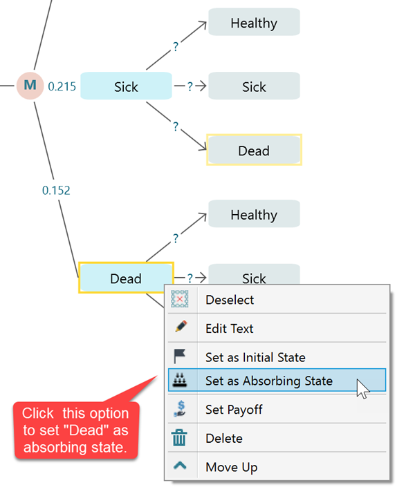
Time-variant probability chart with the X-axis upper bound driven by the maximum number of state transitions set in the Markov simulation settings.

Setting a state as an absorbing state

An absorbing state is one you can never leave once you enter it. The classic example is a "Dead" state: once someone is Dead, they cannot move to "Healthy" or "Sick". In probability terms, an absorbing state has a transition of 1 back to itself and 0 to every other state. When you set the probabilities that way, the software colors that state black to show it is absorbing.

There is a faster way to do this. Just as you set an initial state, select the state, right-click to open the context menu, and choose "Set as absorbing state". The software fills in the right probabilities for you, so you do not have to type the 1 and the 0s yourself.

Right-click context menu on the Dead state in the Markov diagram with the 'Set as Absorbing State' command highlighted to mark Dead as absorbing.

Adding actions to make it a Markov Decision Process

In a Markov Decision Process, you can choose from one or more actions while you are in a given state. For example, in the same chain, you might decide that whenever a patient becomes Sick you can give them either "Treatment A" or "Treatment B", and you want to know which choice leads to the best quality-adjusted life years. The software can work out that policy for you, telling you which action to take in which state.

To set this up, add one or more Markov Action nodes as children of a Markov State node.

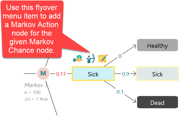
Fly-over menu on a Markov state with the Add Action button highlighted, used to attach Markov Decision Process actions such as Treatment A and Treatment B.

Say you want two actions, Treatment A and Treatment B, for the Sick state. Use that button to create them. Each action gets its own set of transition probabilities and its own payoff, so you can describe how Treatment A behaves and how Treatment B behaves, and then let the software compare them for you.

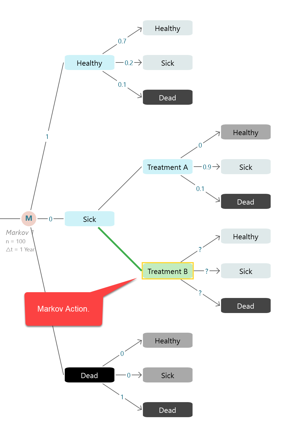
Markov Decision Process diagram showing the Sick state branching into Treatment A and Treatment B action nodes for policy evaluation.

The recommended policy, that is, the best action to take in each state, is shown in the Markov Analyzer panel. So once the model is solved, you can read off the answer at a glance: give Treatment A in this state, Treatment B in that state, and so on.

Setting a reward (or payoff)

Just like adding a payoff to an action or event node in a regular decision tree, you can attach a payoff or reward to a Markov State or a Markov Action. From there you can run a cost-effectiveness analysis on the chain, which is very common in healthcare. For example, you might give the Healthy state a higher quality-of-life value than the Sick state, and give a treatment its yearly cost.

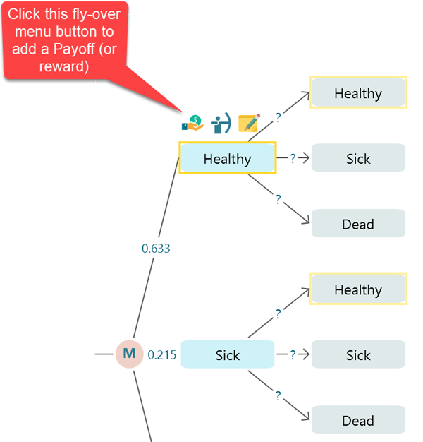
Toolbar Payoff button on a Markov state used to attach a reward or cost-effectiveness payoff to that state.

The screenshot below shows an example that uses QALY and Cost as the payoff. You are not limited to those. You can use DALY or a plain effectiveness variable instead, whichever fits your study. The point is that each state or action carries the numbers your analysis needs, and the software adds them up across all the cycles for you.

Payoff editor for a Markov state configured for cost-effectiveness analysis with QALY as the effectiveness measure and a per-cycle dollar cost.

Fly-over menu on a Markov action node (Surgery) with the Payoff button highlighted by a callout, used to attach a payoff to the action alongside per-state payoffs.

Reading the result charts and tables

Once your model is finished, the software calculates a wide range of useful metrics, charts, and tables and shows them in the Markov Analyzer tab. Expand that tab, as shown below, and you will see results like these. If you want to take a table further, there is an Excel button that exports it for you, so you can keep working with the numbers in a spreadsheet, drop them into a report, or run your own calculations on them.

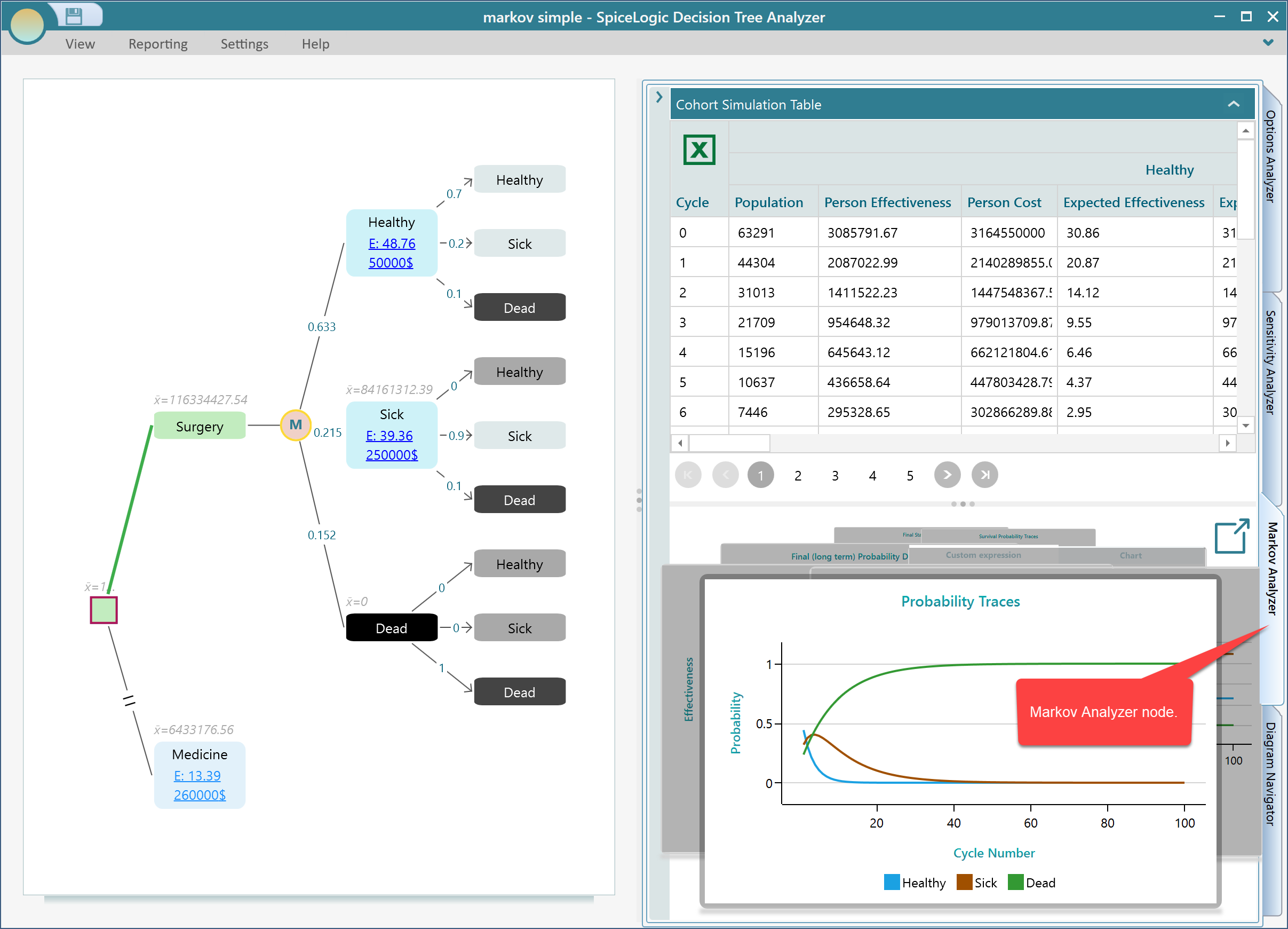
Markov Analyzer panel expanded after the simulation, showing expected metrics, cohort traces, and chart carousel for the selected Markov chance node.

If you would rather see the charts side by side instead of flipping through a carousel, click the Pop-out button to open them all in a separate window. This is handy on a wide screen, or when you want to compare two charts at the same time instead of clicking back and forth.

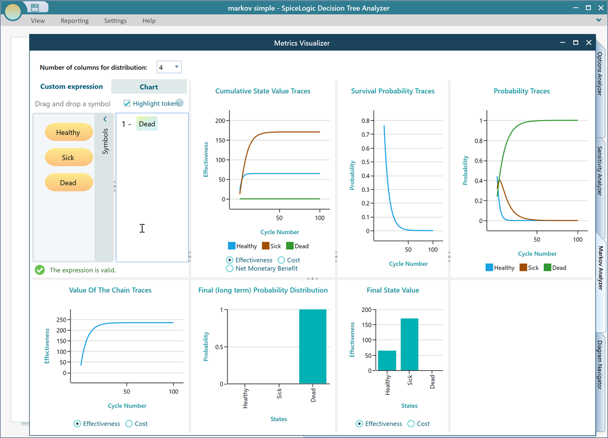
Metrics Visualizer window displaying every Markov chart at once: Cumulative State Value Traces, Survival Probability Traces, Probability Traces, Value of the Chain Traces, Final long-term Probability Distribution, and Final State Value.

Every chart in this software comes with the same handy export tools. Right-click on a chart to open its context menu. From there you can show the data table behind the chart, export that table to Excel, copy the chart image to the clipboard, or save it as an image file. So whether you need the raw numbers or a picture to paste into a slide, it is a couple of clicks away.

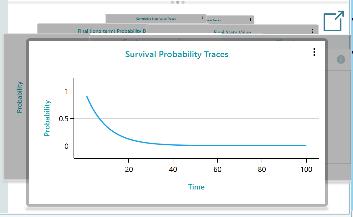
Markov chart with its right-click context menu open (Export Image, Copy Image to Clipboard, Show Data Table, Copy Data Table, Export Data Table to Excel) plus a callout noting that clicking a legend entry can show or hide that series in the chart.

Survival probability

There is a chart dedicated to survival probability. When you have marked a state as absorbing, the software knows that surviving means being in any state other than the absorbing one. So the survival probability is simply the chance of being in any non-absorbing state at each cycle, and the chart plots that over time. If your absorbing state is "Dead", this chart shows the share of the group still alive at each cycle, which is exactly the survival curve you would expect to see.

Custom state expression

Sometimes you want to ask a question the built-in charts do not answer directly, such as "what is the chance of being in State A or State B, but not State C?". The software lets you write a custom expression for exactly that kind of query, and then it draws a chart based on your expression. Just select Custom Expression in the carousel.

As an example, even though there is already a dedicated survival probability chart, imagine there was not one. You could model the survival probability yourself with a custom expression and watch it over the cycles. It is a flexible way to combine states however your question needs.

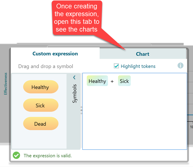
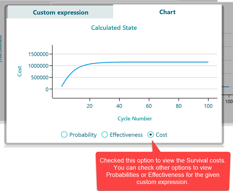
Custom Expression editor with draggable state symbols (Healthy, Sick, Dead) and a sample expression (Healthy + Sick), used to combine Markov states for charting; callout points to the Chart tab.

Once you open the Chart tab, you can choose what the custom expression should plot: the probability traces, the costs, or the effectiveness of being in those states. So the same expression can show you how likely those states are, what they cost you, or how much benefit they bring, depending on what you pick.

Chart tab for a custom Markov expression showing the Calculated State Cost curve over cycle number, with Probability, Effectiveness, and Cost radio options to switch the plotted metric.

Discounting the Markov cycle payoff

Money and benefits in the future are usually worth less than the same amount today, and you can account for that with an interest rate. Set an interest rate, and every future Markov cycle payoff is discounted by it. You set this in the Cost-Effectiveness Criterion editor, which has a section at the bottom for discounting interest rates.

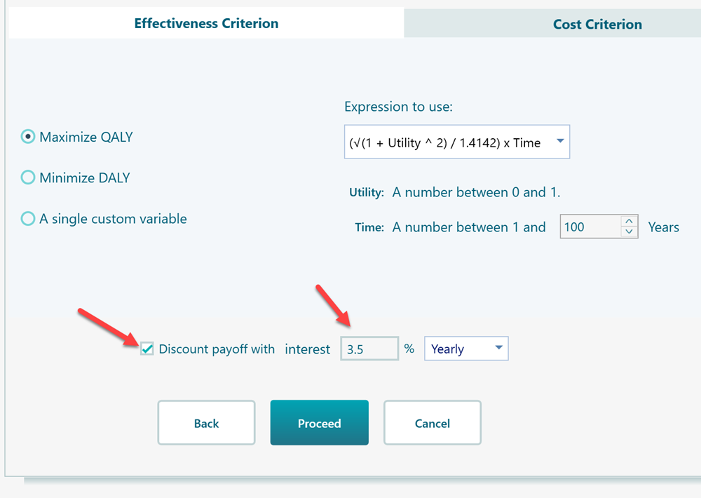
Cost-Effectiveness Criterion editor in Decision Tree Analyzer showing the interest rate field used to discount future Markov cycle payoffs.

If you set that box to an interest rate greater than 0, each Markov cycle is treated as a future event. The software works out the year of the event from the Markov cycle duration, and then discounts that cycle's payoff accordingly. So a longer cycle duration pushes payoffs further into the future and discounts them more. For example, at a 3% rate, a benefit earned 10 years out counts for less than the same benefit earned next year, just as you would expect in a real cost analysis.

Wrapping up

That covers the main pieces of Markov modeling in the Decision Tree software. The best way to get comfortable is to build a small model of your own and click around. Start with three states, set a few probabilities, add a payoff, and run it. Try the features for yourself, and you will quickly find handy ways to put them to work.

Modeling Markov Chain and Markov Decision Process