Custom Discrete Distribution

A discrete distribution is one where the random variable can only land on separate, countable values. Think of the roll of a die, which can be 1, 2, 3, 4, 5, or 6. Or the number of customers who walk in tomorrow, which could be 0, 1, 2, and so on. There is nothing in between. You never get a 2.5 on a die. This is different from a Custom Continuous Distribution, where the variable can take any value across a range, like a height of 1.732 meters.

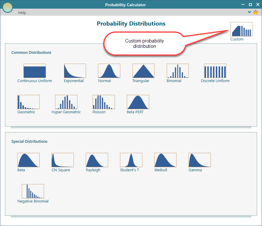
The app already comes with the common probability distributions built in, and most of the time one of those will fit your needs. But every now and then your situation does not match any of them. Maybe you ran your own survey, or you worked out a rule by hand, and you just want to enter those numbers directly. That is exactly what a custom discrete distribution is for. You define the shape yourself.

To start, open the dashboard and click the 'Custom' button.

Using Piecewise Expressions

One way to build a custom distribution is with a piecewise expression. "Piecewise" just means the formula changes depending on the value of x. You write one rule for one range of values and a different rule for another. This is handy when your probabilities follow a formula rather than a fixed list of numbers.

Here is a quick example. Say the probability is one value when x is below 5, and a different value when x is 5 or higher. Each piece covers its own slice of the range. The app reads x, checks which condition it falls under, and uses the matching rule.

In this section we will walk through how this works for a discrete distribution, step by step.

To begin, select the piecewise option as shown below.

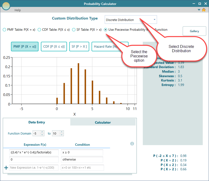
Look at the Data Entry tab in the screenshot above. This is where you type an expression using the variable 'x'. Each line is one expression for one condition.

If you only have a single line, you do not need a condition at all, so you can leave the condition box blank. That one expression then applies to the whole range. But once you have more than one line, each line needs its own condition. Without that, the app would have no way to know which expression to use for which value of x.

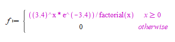
The expression in the screenshot above reads as follows.

The probability mass function of this custom distribution is:

The expression editor can handle a lot more than simple formulas. You can use math functions, operators, and much more. To see the full list of what it supports, read about the Custom Expression Editor.

Function Domain

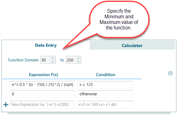
When you write a piecewise expression, you also need to tell the app the domain of the function. The domain is just the range of values that x is allowed to take. You set it by entering a Minimum value and a Maximum value for the function.

Setting the domain matters because it tells the app where your distribution starts and where it stops. For example, if you are modeling a dice roll, the minimum would be 1 and the maximum would be 6. Anything outside that range gets a probability of zero.

Using a Data Points Table

If you do not have a formula, the quickest way to define a distribution is often a table. You simply list each possible value of the random variable next to its probability. This is a natural fit when your numbers come from real data, like a survey result or a count of past outcomes.

The app gives you three ways to enter this table. You can type in the Probability Mass Function directly, or you can use the Cumulative Distribution Function, or the Survival Function. Pick whichever form your data already comes in, and the app takes care of the rest.

Table for the Probability Mass Function

The Probability Mass Function, or PMF, is the most direct of the three. It is just a table that lists the probability of each single outcome. For a fair die, for example, each of the six faces would get a probability of about 0.167.

To enter your distribution this way, select the PMF radio button as shown below, then fill in the table.

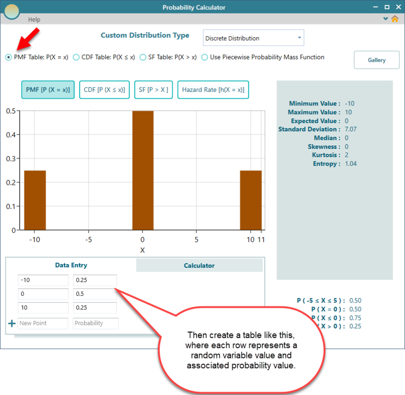
Table for the Survival Function

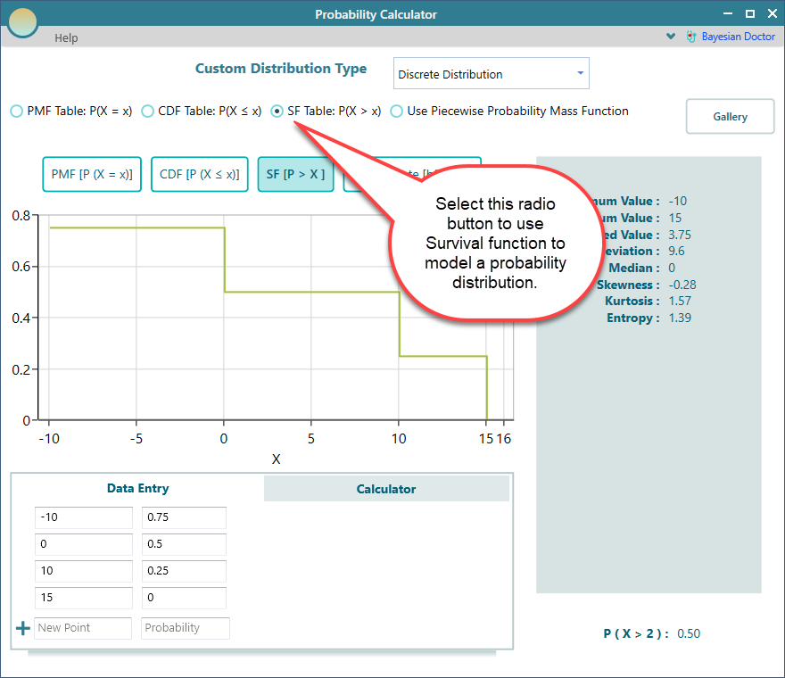
You can also define your distribution with a Survival Function table. The Survival Function gives the probability that the outcome is greater than a given value. In other words, it is the chance of "surviving" past that point. This form shows up a lot in reliability and lifetime studies. A good example is the probability that a machine is still running after a certain number of hours.

Entering it works just like the PMF table. Check the radio button for the SF table and type in your data.

We have a separate page that goes deeper into Modeling with the Survival Function. Have a look there for a full walkthrough.

Table for the Cumulative Distribution Function

The PMF and the Survival Function are not your only options for a data table. You can also work from the Cumulative Distribution Function.

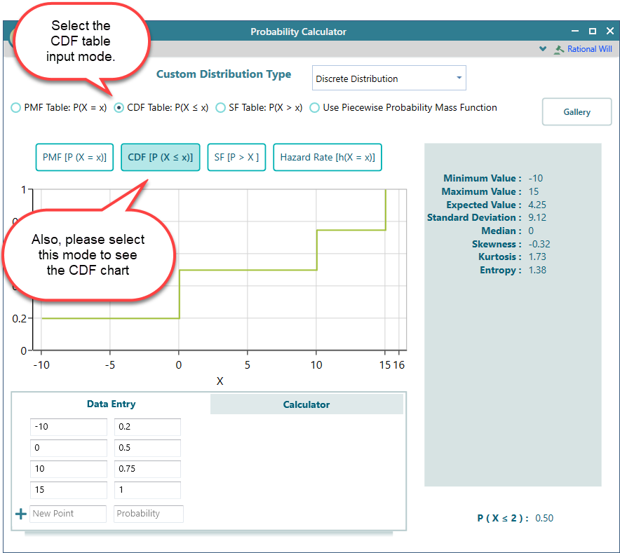
The Cumulative Distribution Function, or CDF, gives the probability that the outcome is less than or equal to a given value. So instead of the chance of each separate result, it adds them up as you move along, building toward a total of 1. If your data already comes in this running-total form, this is the easiest table to use.

Select the CDF table radio button as shown below.

We have a separate page with the full details on Modeling the Cumulative Distribution Function. Check it out to learn more.

Scaling

No matter how you define your custom distribution, whether with a data point table or an f(x) expression, there is one rule every probability distribution has to follow. All of the probabilities must add up to exactly 1. This makes sense, because something has to happen, so the chances of all possible outcomes together have to cover 100 percent.

The good news is you do not have to get this exactly right yourself. If your numbers do not quite sum to 1, the app automatically scales your Probability Mass Function so that they do:

∑ PMF(X = x) = 1

Every property and calculated value the app reports is based on this scaled function, not on your raw input. So you can enter your data in whatever form is convenient, and the app handles the normalizing for you.