Bernoulli Utility Function

Same as an exponential utility function or any other utility function, you can use a Bernoulli utility function to associate a payoff in your decision tree. In this tutorial, you will learn basically what is a Bernoulli utility function, and how to use a Bernoulli Utility function in a decision tree.

What is the Bernoulli Utility Function?

Bernoulli suggests a form for the utility function in terms of a differential equation. He proposes that marginal utility is inversely proportional to wealth. If total wealth is expressed as W, and the utility function is U(W), then

Like any proportional expression, we can introduce a constant and express with an equal sign. let's call this constant "a".

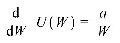
What is exactly the Marginal Utility?

Marginal utility is an expression of how the Utility value changes for each additional unit of gain. If you are familiar with calculus, then you know that differential operation is the math operation that gives us any expression's rate of change. So, here, we used the differential operator . Let me give you an example. Say, you have 50$ in your pocket, how much more excited will you feel if you just get 1$ (so your total wealth will be 51$)? hmm, maybe someone will be somewhat excited. Say, that excitement value is "10". Now, say,  you have 100,000$ in your pocket. If you get 1$ on top of that your net wealth will be 100,001$. How much excited will you feel? Not sure about everyone, but most rational people will feel the "0" temptation to get that 1$ when the 100,000$ he or she has in his/her pocket. So, you can understand that the more wealth is gained, the temptation to get an extra 1$ gets diminished. but, when the net wealth is very low, the extra 1$ gets much more exciting. That is the idea of marginal utility of the Bernoulli Utility Function.

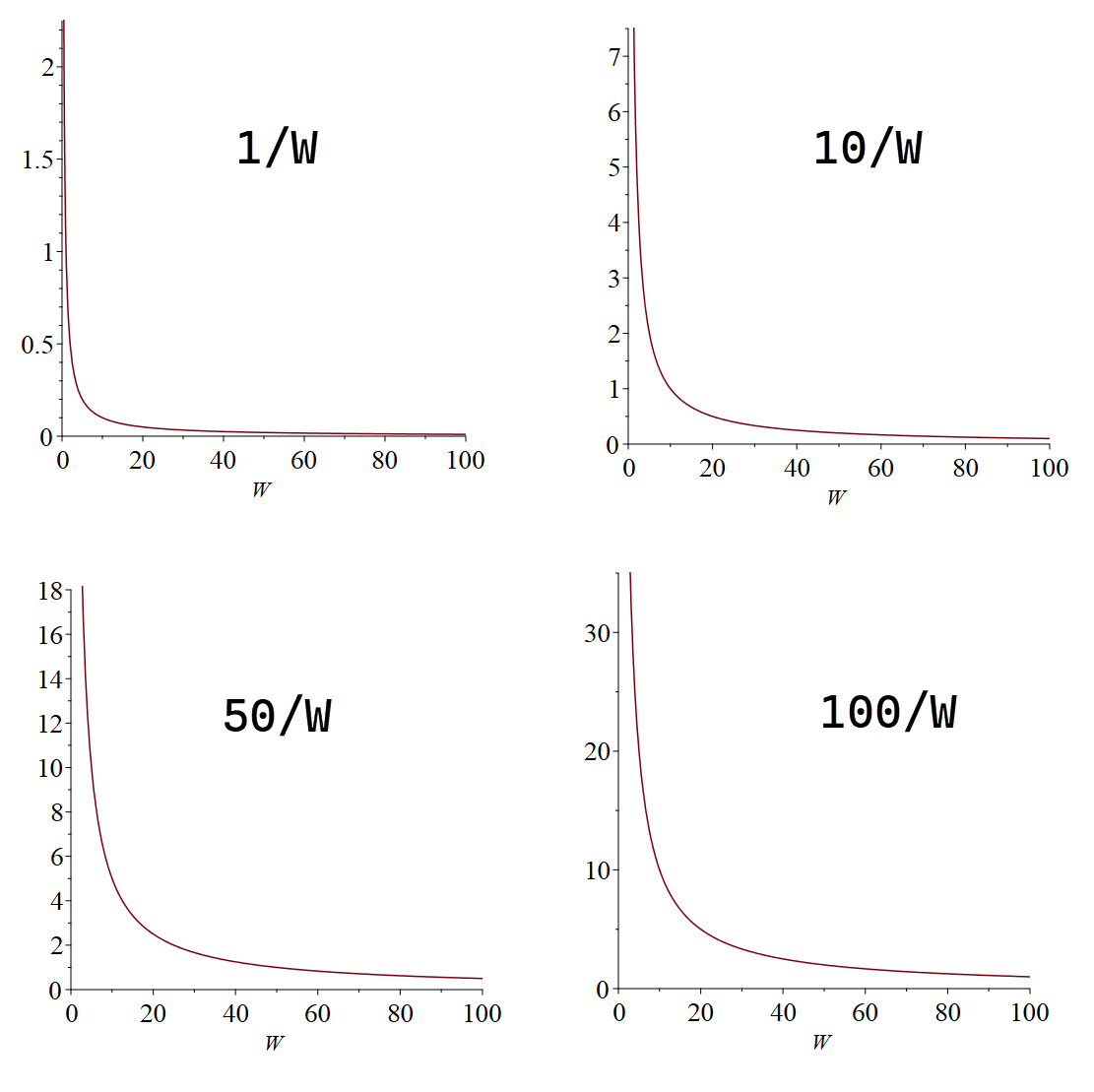
In our expression, we introduced a proportional constant "a". This "a" value can be anything to reflect a specific person's situation. You can fine-tune this value "a" to match someone's net wealth and model his/her utility function. We will show how to calculate this constant in this tutorial. Now, if we plot this expression for various "a" value as "a" = 1, "a" = 10, "a" = 50, "a" =100, we observe a pattern.

We can solve this differential equation to find the function "U(W)". By solving the differential equation by integrating both sides, we get

So, after solving the differential equation, we get another constant "b". We can now use "a" and "b" to scale the utility function to fit any specific scenario. These constants "a" and "b" are called scaling parameters.

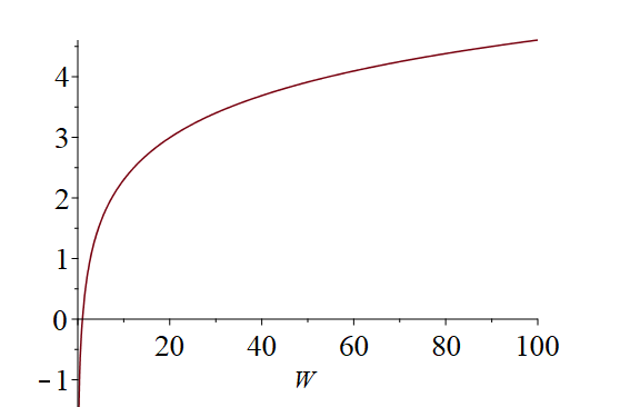
Say, a = 1 and b = 0, we see the function plots like this.

What does it mean by scaling parameters?

Say, you want your utility function such that, for a given scenario, the maximum possible payoff should give U(maximum payoff) = 1. and the minimum payoff should be U(minimum payoff) = 0. Using some parameters, you can adjust the utility function in that way. These parameters are called scaling parameters.

You can determine the value of "a" and "b" like this.

Set any value to W, i.e. 100, and ask yourself, what is your utility value for that wealth? You get a number. (i.e. 0.1 Utils) Put that number in the above equation.

Then, set another value to W, i.e. 1000 or whatever you like, then ask yourself again, what is your Utility value for such high wealth? You will get another number. (i.e. 0.9). Then, you will get 2 equations where the variables are just "a" and "b". When you have 2 equations with 2 variables, using linear algebra, you can solve the value for those variables, right? So, you will get "a" and "b" accordingly.

Solving these 2 linear equations, we get,

Our Decision Analysis Software (Decision Tree Software or Rational Will) can calculate that parameter based on the Minimum and Maximum possible values in the decision context, which is collected from the user.

Risk Aversions

According to behavioral economics, the mathematical expression of the absolute risk aversion for any utility function is defined as:

Applying the above operation to the Bernoulli utility function, we get the absolute risk aversion as:

The relative risk aversion formula for any utility function is defined as:

Applying the above formula, we can get the relative risk aversion for a Bernoulli utility function as

Modeling Example

Say, you have two business opportunities and you want to decide which one is best. They are Investment A and Investment B. Investment A can bring 20,000$ in revenue with a probability of 0.2 and 500$ with a probability of 0.8. Investment B can bring 2000$ with a probability of 0.85 and 100$ with a probability of 0.15.

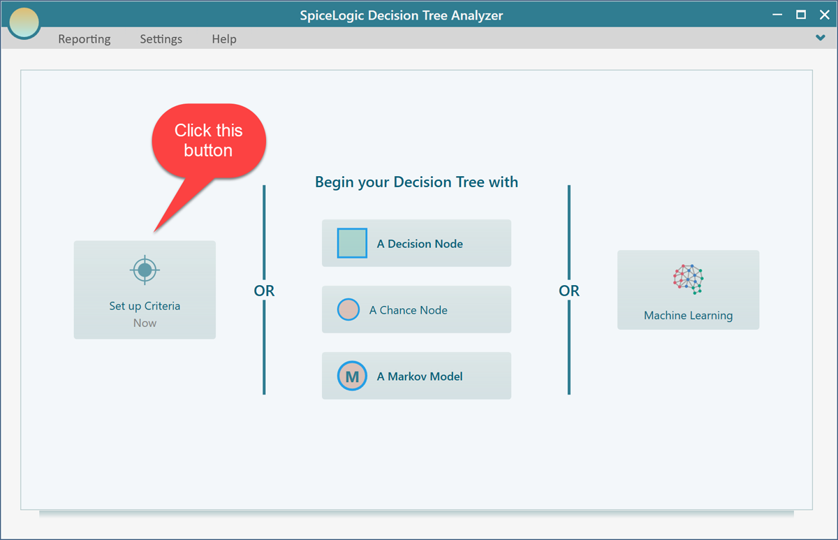
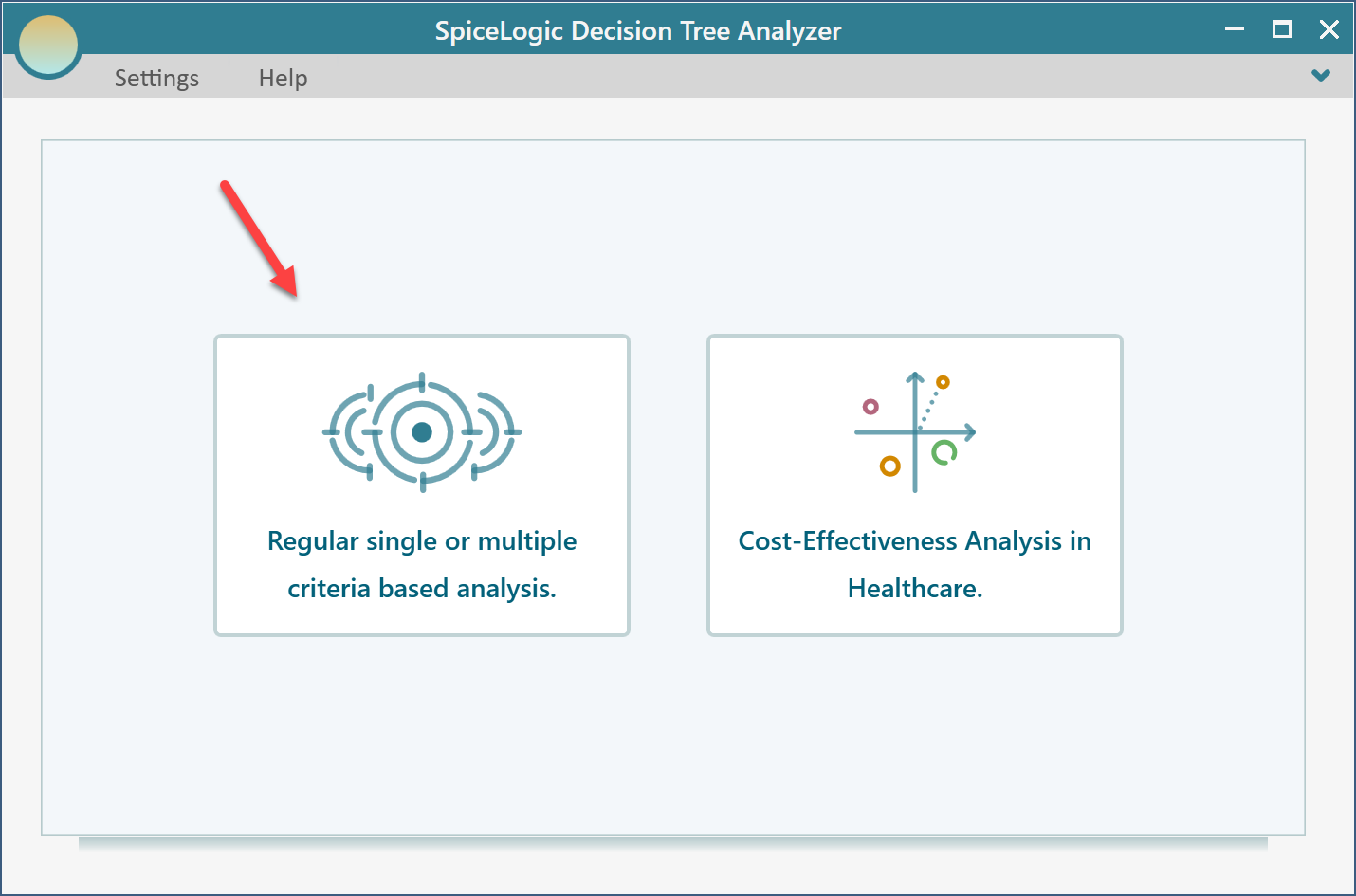
If you are using the Decision Tree Analyzer software then you will be greeted with the following screen. If you are using Rational Will software, click the "Decision Tree" button from the home screen to get to this view. Click the button "Set up Criteria".

Once you click that button, you will be asked, if you want to use a regular single/multiple criteria analysis or a Cost-Effectiveness analysis. Choose the first option. 

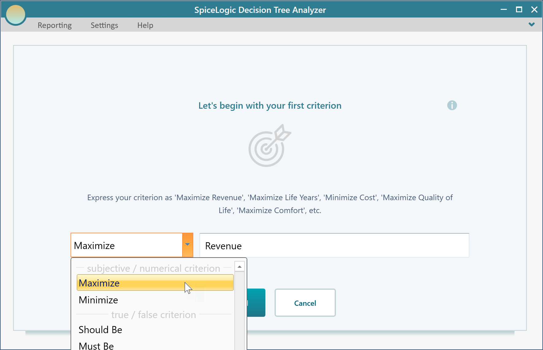
Then you will be presented with the following screen. Select "Maximize" and enter "Revenue" as shown below. 

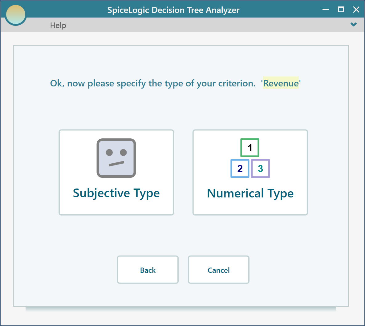
Then click the "Proceed" button. You will be asked about the type of criterion. Select "Numerical Type". Please remember that, in order to use a Utility function, you need to use the Numerical type criterion.

Then you will be asked about the minimum and maximum payoff range from the investment. Enter Minimum = 100$ and maximum = 20,000$

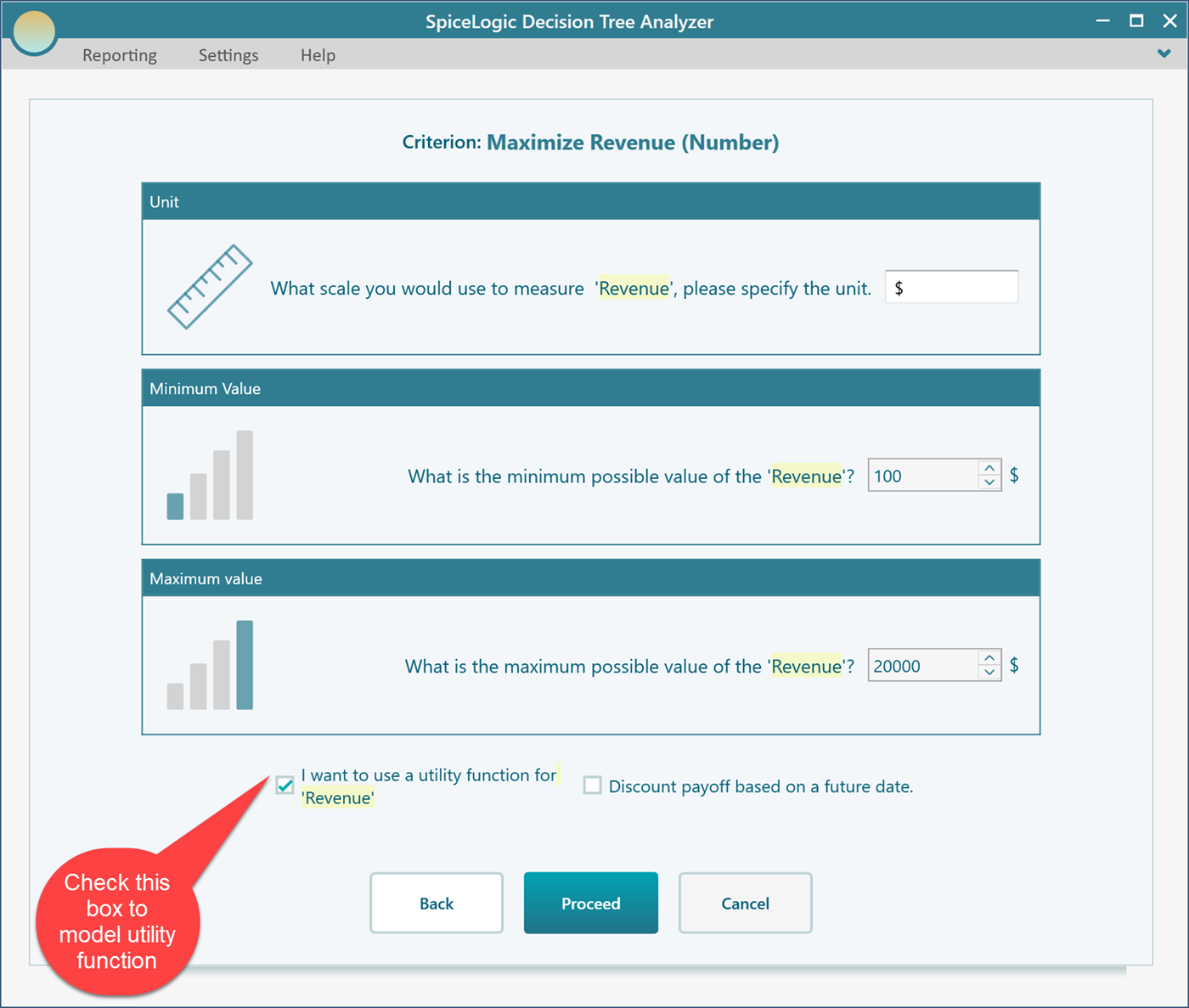
Click Proceed. As you have checked the box "I want to use a utility function...", you will be presented with a utility function editor. Select the "Bernoulli Utility Function" button.  

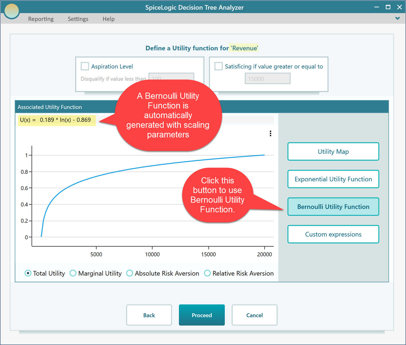
How Scaling parameters are calculated

You may be curious, in the generated utility function, from where these scaling parameters are 0.189 and -0.869 come. The scaling parameters are calculated such that, the maximum payoff will result in the highest utility value which can be 1 or 100, depending on the preference. The lowest payoff will result in the lowest utility value which can be 0, -1, or -100, depending on the preferences as well. The preference can be specified from the ribbon as shown here. 

Viewing other derivatives of the generated utility function.

You can check the Marginal Utility function, Absolute Risk Aversion, and Relative Risk Aversion from the radio buttons as you can see at the bottom of the panel. Here is the Marginal Utility Function for the above-generated function.

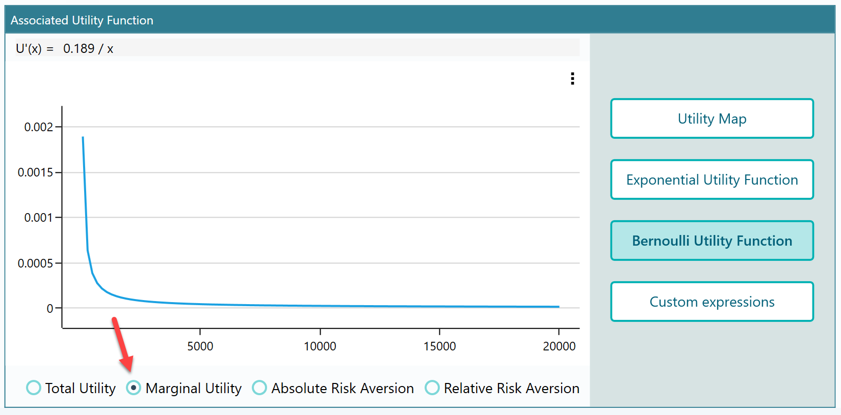
Finally, model the Decision Tree

Click Proceed button. Then, you will be asked if you want to add another criterion. Click "No".  

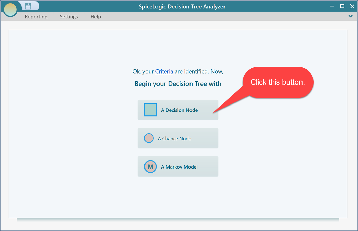
Then, click the "decision Node" button to create a decision tree with a Decision Node as the root node.

Then, create a decision tree like this. If you are not familiar with how to create the decision tree in our decision tree software, please visit the getting started page. From that page, you will know how to set a payoff to a node.

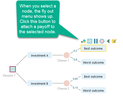
Then, set the payoff for each node.

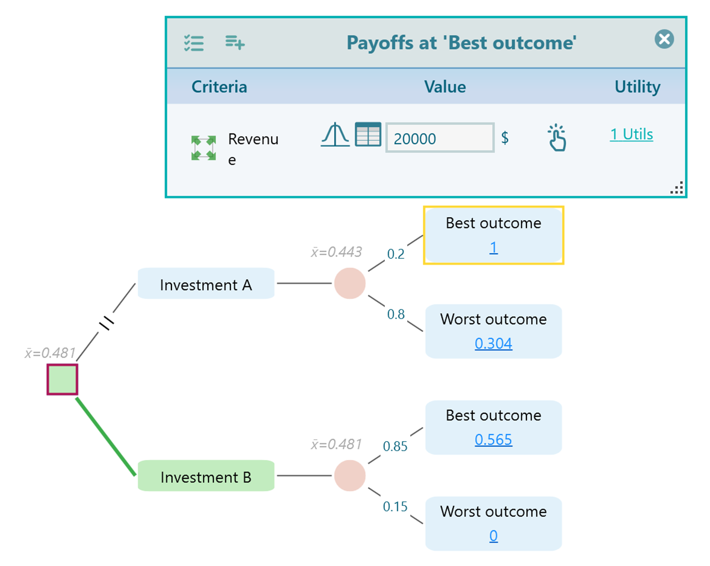
Anytime, you click the Utility value link shown on each node, the Payoff editor will show up.

Within the payoff editor, click the Utils link to open the utility function chart. You can also see a green vertical line that indicates where your utility stands in the plot based on the currently set payoff. The line moves as you change the payoff instantly.

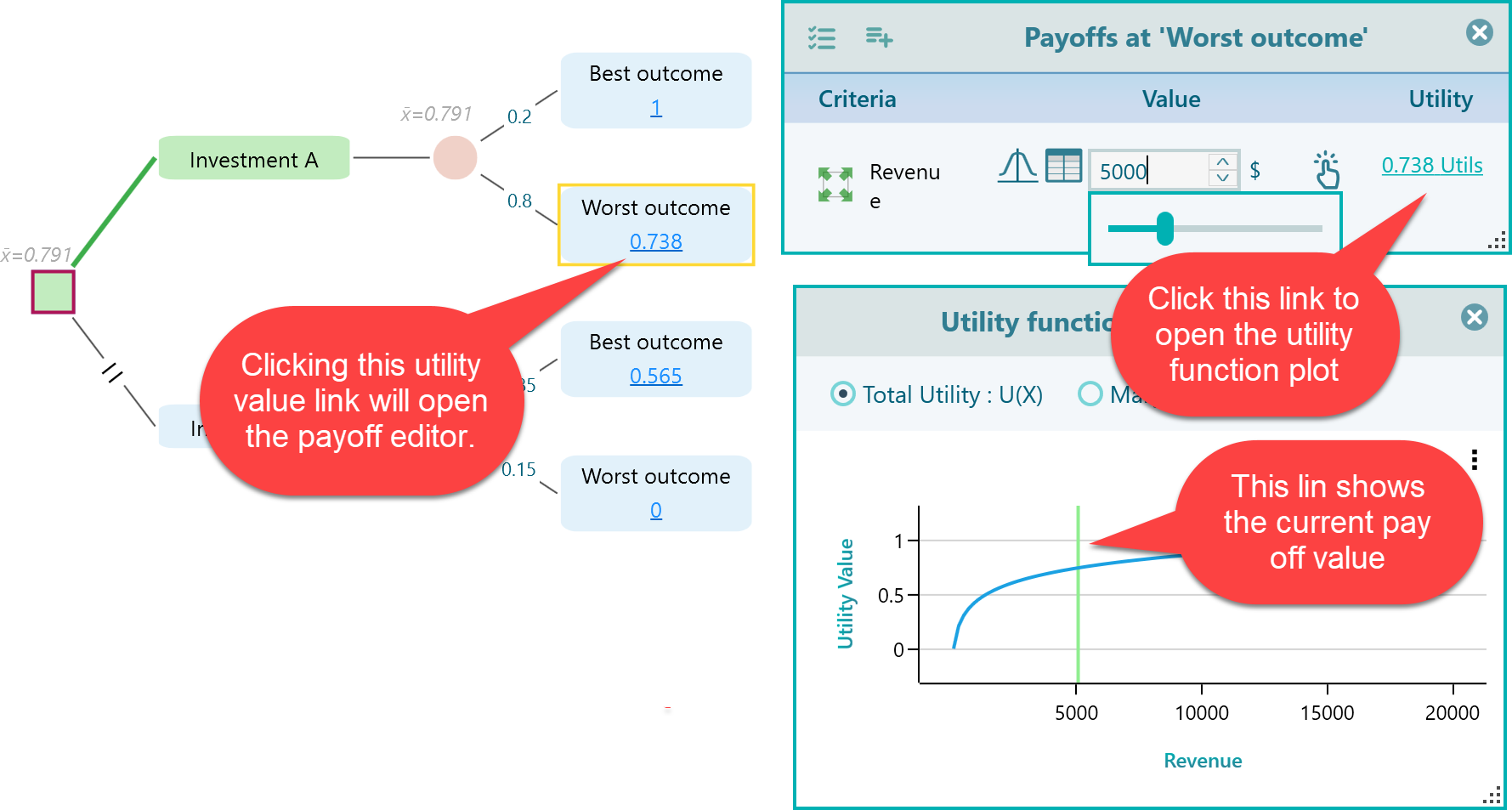
The constraint of a Bernoulli Utility Function

Even though the Bernoulli Utility function can model realistic behavior very well, there is a minor detail that needs to be remembered when using such an equation.

What is the natural logarithm of zero?

 is undefined.

Since ln(0) is the number that we get by solving the equation:

There is no value of x that satisfies this equation.

So, for a value of x, your Bernoulli Utility Function will give a value that is undefined.

If your payoff's Minimum and Maximum value is such a range where 0 can be a possible number, then our software will show an error.

In order to avoid such a problem, we recommend setting the Minimum Payoff value greater than 0.