


Bernoulli Utility Function
Just like the exponential utility function, or any other utility function, you can attach a Bernoulli utility function to a payoff in your decision tree. This tutorial keeps things simple. First you will learn what a Bernoulli utility function is and why people use it. Then you will see, step by step, how to apply one inside a decision tree.
What is the Bernoulli Utility Function?
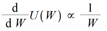
Bernoulli described the utility function as the answer to a small differential equation. His idea was that marginal utility is inversely proportional to wealth. In plain words, the richer you already are, the less an extra dollar means to you. If we write total wealth as W and the utility function as U(W), that idea looks like this:
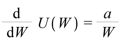
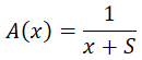
When one thing is proportional to another, we can turn it into a normal equation by adding a constant. Let's call that constant "a". With the constant in place, we can swap the proportional sign for an equals sign and get this:
What exactly is marginal utility?
Marginal utility tells you how much the utility value changes for each extra unit you gain. If you have done any calculus, you will recognize this as a rate of change. The differential operator is the math tool that gives us the rate of change of an expression. That is why the equation above uses it.

Here is a simple example. Say you have $50 in your pocket. How happy would one more dollar make you, taking you to $51? Probably a little happy. Let's put a number on that happiness and call it "10". Now imagine you have $100,000 in your pocket. One more dollar takes you to $100,001. How excited are you now? For most people, almost not at all. The point is easy to feel. The more wealth you already have, the less an extra dollar tempts you. When you have very little, that same extra dollar feels much bigger. That is the heart of marginal utility in the Bernoulli utility function.
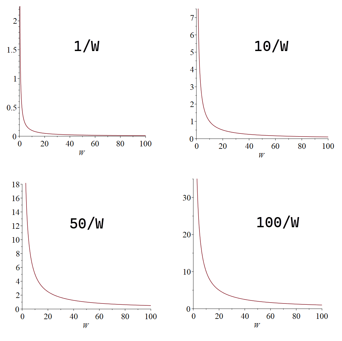
Notice the constant "a" we added earlier. You can set "a" to whatever value fits a person's situation, so the same equation can describe a careful saver or a high roller. Later in this tutorial we will show how to work out the right value for it. For now, if we plot the expression for a few different values, say a = 1, a = 10, a = 50, and a = 100, a clear pattern shows up.
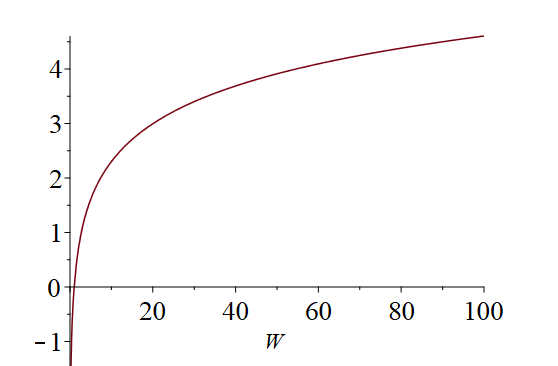
We can solve this differential equation to find the function "U(W)". Integrating both sides gives us this result:
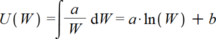
Solving the differential equation leaves us with a second constant, "b". So now we have two constants, "a" and "b". Together they let us stretch and shift the utility function to fit any situation we care about. These two constants are called the scaling parameters.
For example, with a = 1 and b = 0, the function plots like this:
What do the scaling parameters actually do?
Suppose you want a utility function where, for a given decision, the best possible payoff scores U = 1 and the worst possible payoff scores U = 0. The scaling parameters are what let you line the function up that way.
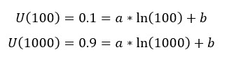
Here is how you find "a" and "b". Pick any wealth amount, say 100, and ask yourself how much that is worth to you on a utility scale. You get a number, say 0.1 utils. Put that pair into the equation. Now pick a second amount, say 1000, and ask the same question. You get another number, say 0.9. You now have two equations, and the only unknowns in them are "a" and "b". Two equations with two unknowns can be solved with basic linear algebra, which gives you the exact values of "a" and "b".
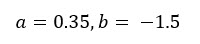
Solving those two equations gives us:
You do not have to do this by hand. Our decision analysis software (Decision Tree Software or Rational Will) works out those parameters for you. It uses the smallest and largest possible values in your decision, which it collects from you as you set things up.
Risk Aversion
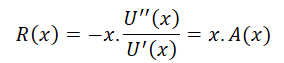
In behavioral economics, the absolute risk aversion of any utility function is written like this:
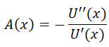
Applying that formula to the Bernoulli utility function gives us the absolute risk aversion:
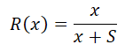
The relative risk aversion of any utility function is written like this:
Applying that formula to the Bernoulli utility function gives us the relative risk aversion:
A Worked Example
Imagine you have two business opportunities and you need to pick one. Call them Investment A and Investment B. Investment A pays $20,000 in revenue with a probability of 0.2, and $500 with a probability of 0.8. Investment B pays $2,000 with a probability of 0.85, and $100 with a probability of 0.15. Which one should you choose? On a simple average, Investment A looks bigger, but it is also far riskier, since most of the time it pays only $500. A utility function is the right tool for a choice like this, because it weighs the risk and not just the average. Let's set it up in the software.
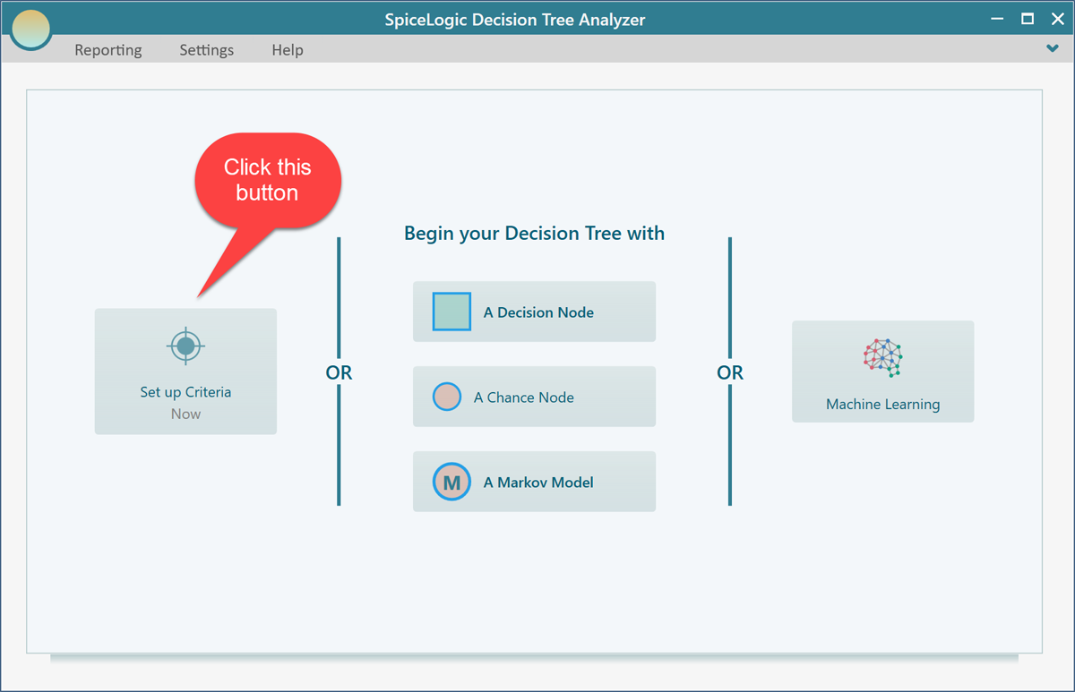
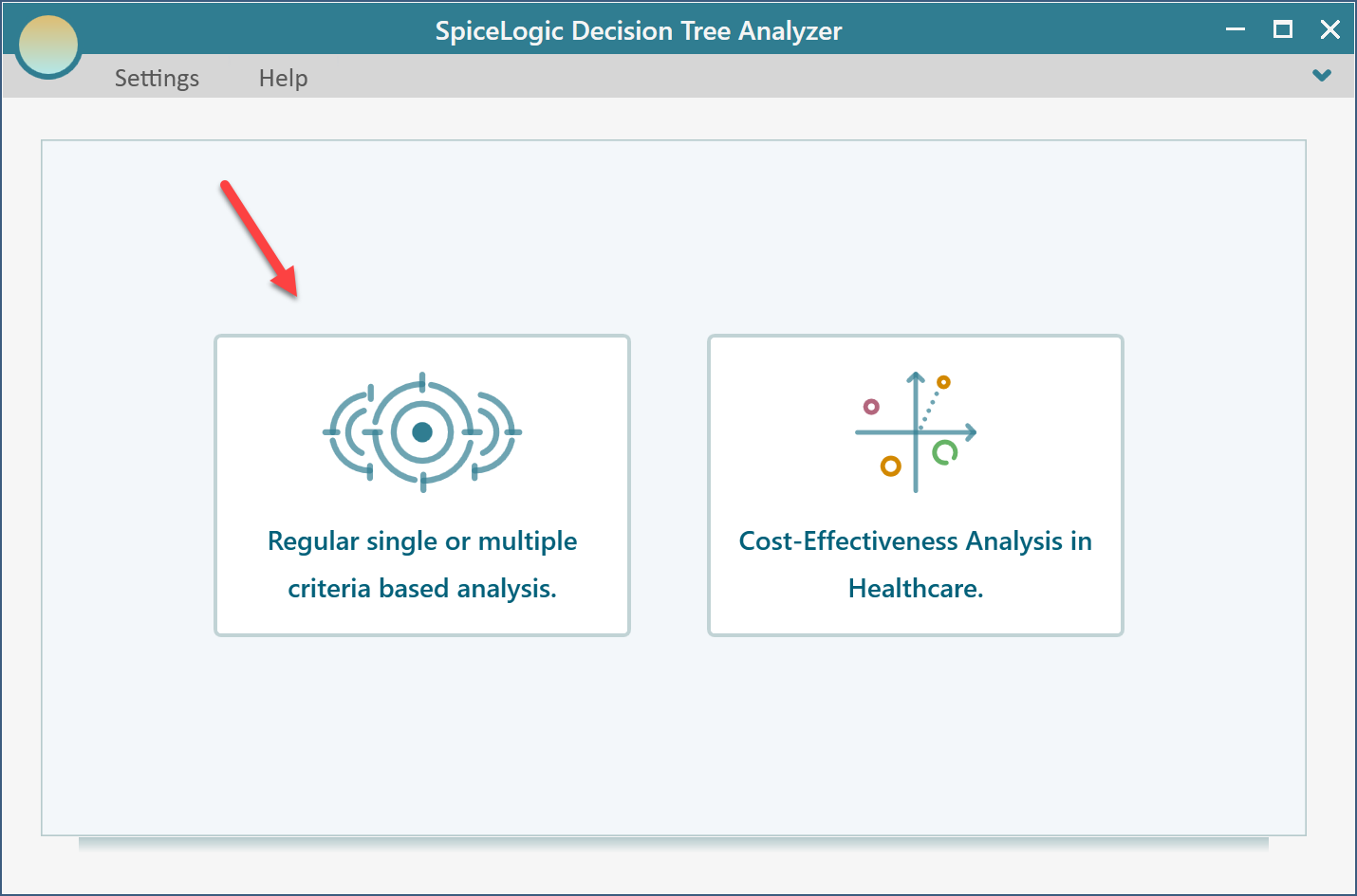
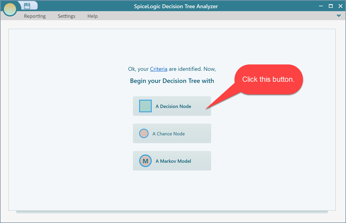
If you are using the Decision Tree Analyzer, this is the first screen you will see. If you are using Rational Will, click the "Decision Tree" button on the home screen to reach the same view. Now click the "Set up Criteria" button.
The software now asks whether you want a regular single or multiple criteria analysis, or a Cost-Effectiveness analysis. Choose the first option.
The next screen asks how to handle your criterion. Since more revenue is better, select "Maximize" and type "Revenue", as shown below.
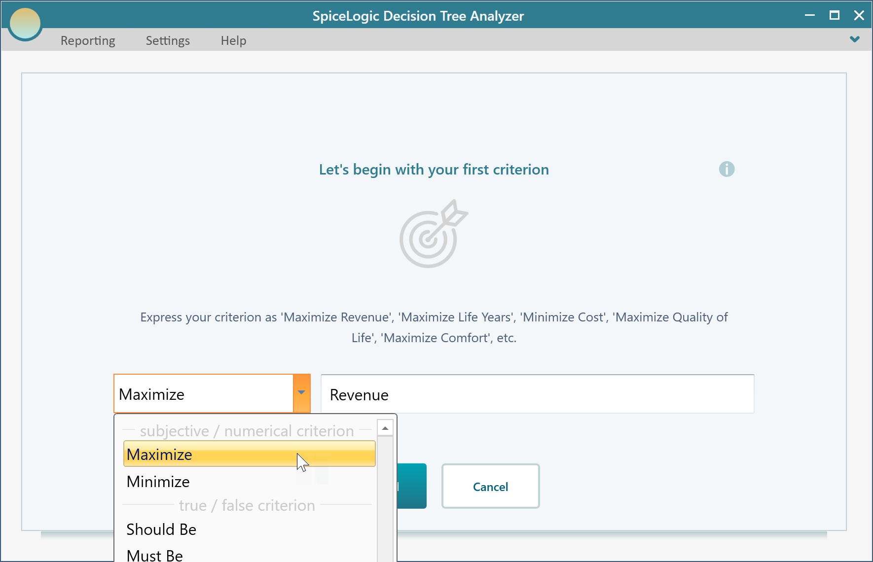
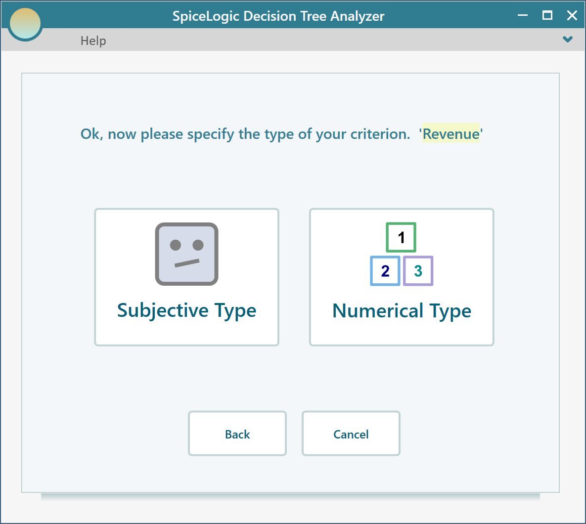
Click the "Proceed" button. The software then asks for the type of criterion. Select "Numerical Type". This step matters. A utility function only works with a numerical type criterion, so be sure to pick it here.
Next, the software asks for the range of payoffs you could get from the investment, the smallest and the largest. Enter Minimum = $100 and Maximum = $20,000. On this same screen, check the box that says you want to use a utility function, so the editor appears in the next step.

Click Proceed. Because you checked the "I want to use a utility function..." box, the software now shows you the utility function editor. Click the "Bernoulli Utility Function" button.
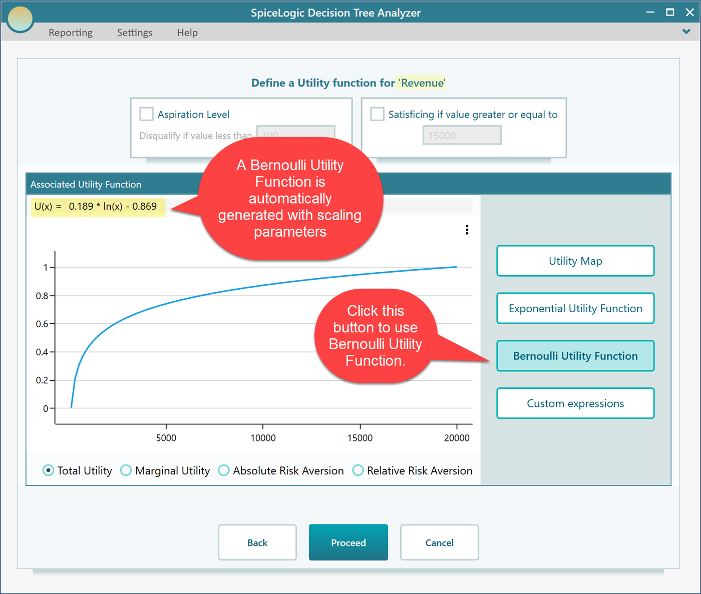
Where the scaling parameters come from
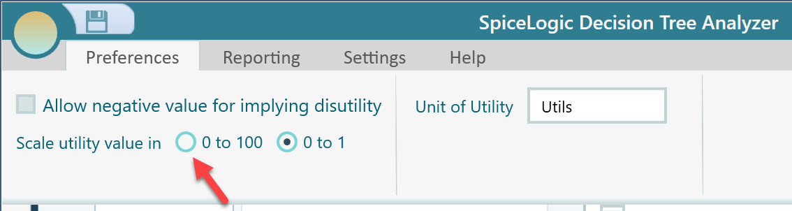
You might wonder where the scaling parameters in the generated function, 0.189 and -0.869, came from. The software picks them so that the highest payoff lands on the top of your utility scale and the lowest payoff lands on the bottom. The top can be 1 or 100, and the bottom can be 0, -1, or -100, depending on which scale you prefer. You set that preference from the ribbon, as shown here.
Viewing the other curves derived from your utility function
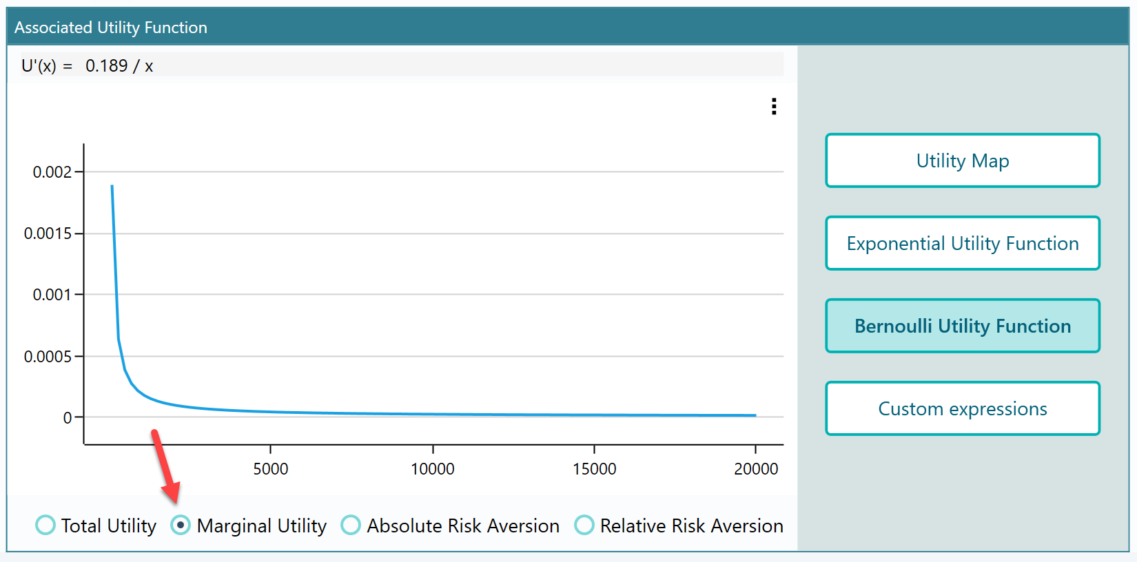
From the radio buttons at the bottom of the panel, you can also look at the Marginal Utility function, the Absolute Risk Aversion, and the Relative Risk Aversion for the function you just generated. These are handy when you want to see how your attitude to risk changes across the payoff range, not just the utility value itself. Here, for example, is the Marginal Utility function for it.
Now build the decision tree
Click the Proceed button. The software asks whether you want to add another criterion. Since we only care about revenue here, click "No".
Then click the "Decision Node" button to start a decision tree with a Decision Node as its root.
Now build out a decision tree like the one below. If you have not created a decision tree in our software before, take a look at the getting started page first. It walks you through the basics, including how to set a payoff on a node.
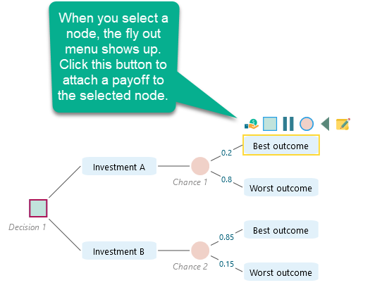
Next, set the payoff for each node.
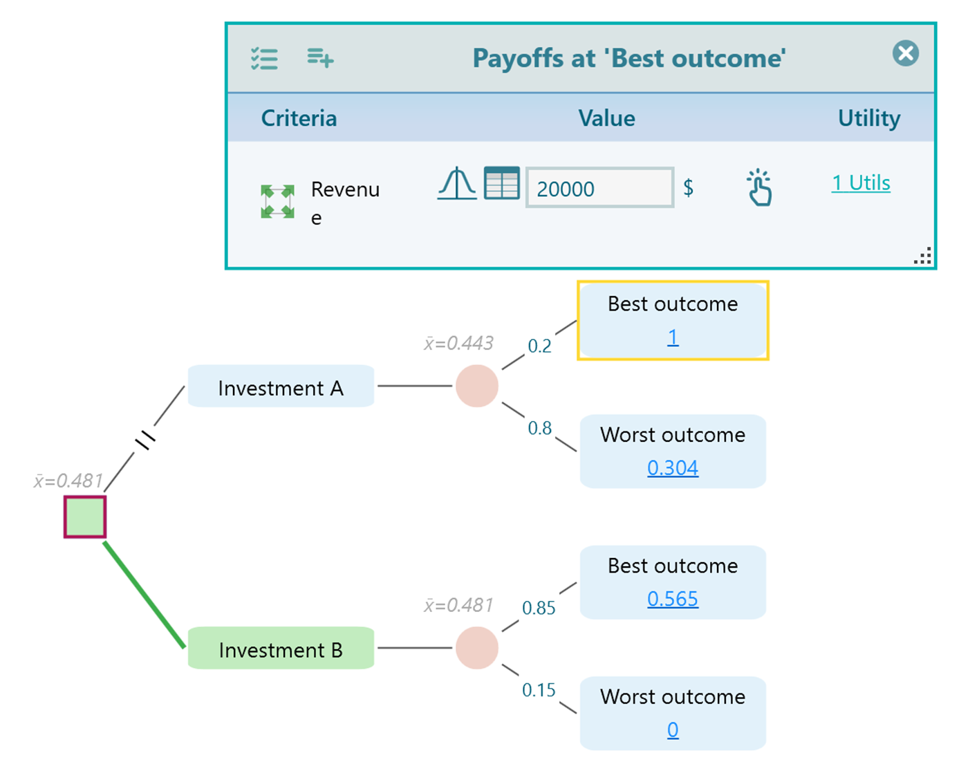
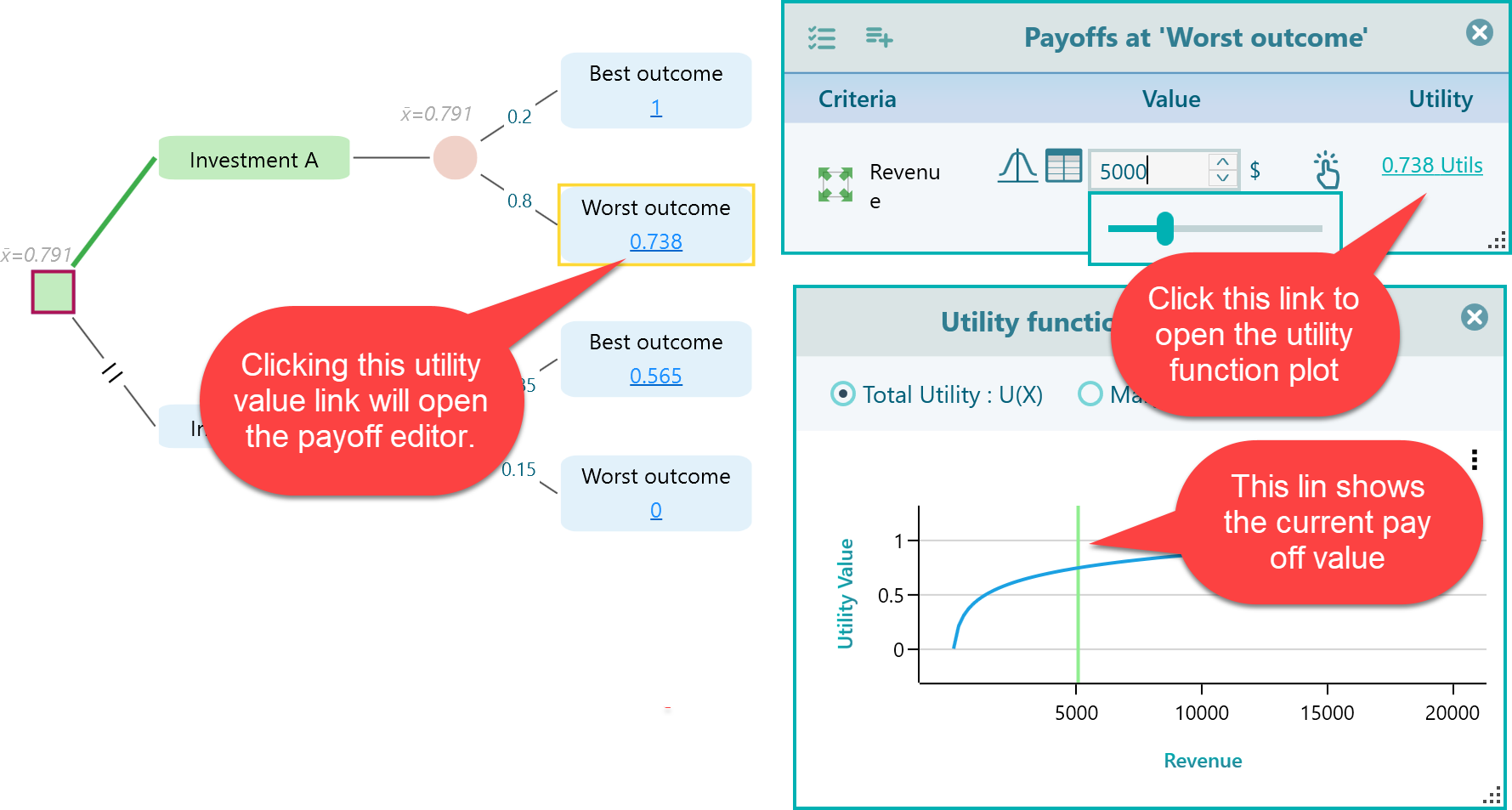
Whenever you click the Utility value link on a node, the Payoff editor opens.
Inside the Payoff editor, click the Utils link to open the utility function chart. You will see a green vertical line that marks where your current payoff sits on the curve. As you change the payoff, the line slides along the curve right away, so you can watch your utility move as you type. It is a quick way to sanity check a payoff before you trust the result.
One thing to watch with the Bernoulli Utility Function
The Bernoulli utility function does a good job of describing how people really value money, but there is one small detail to keep in mind when you use it.
What is the natural logarithm of zero?

The answer is that it is undefined.
Here is why. The value ln(0) would be the number x that solves this equation:

No value of x makes that equation true. So the natural logarithm of zero simply has no answer.
Because the Bernoulli utility function uses a logarithm, a payoff of zero gives an undefined result. If your payoff range includes zero as a possible value, the software will show an error. To avoid this, keep your minimum payoff above zero. For example, instead of a low payoff of $0, use a small positive number like $1. The result barely changes, and the function stays well defined.