All articles

Is Riding Without a Ticket a Winning Bet? A Kitchen-Table Decision Tree

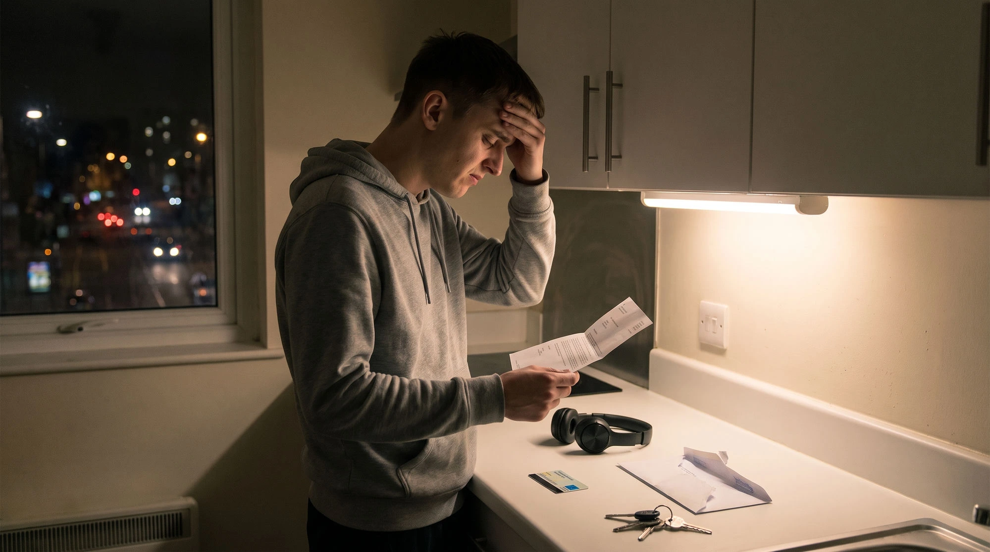
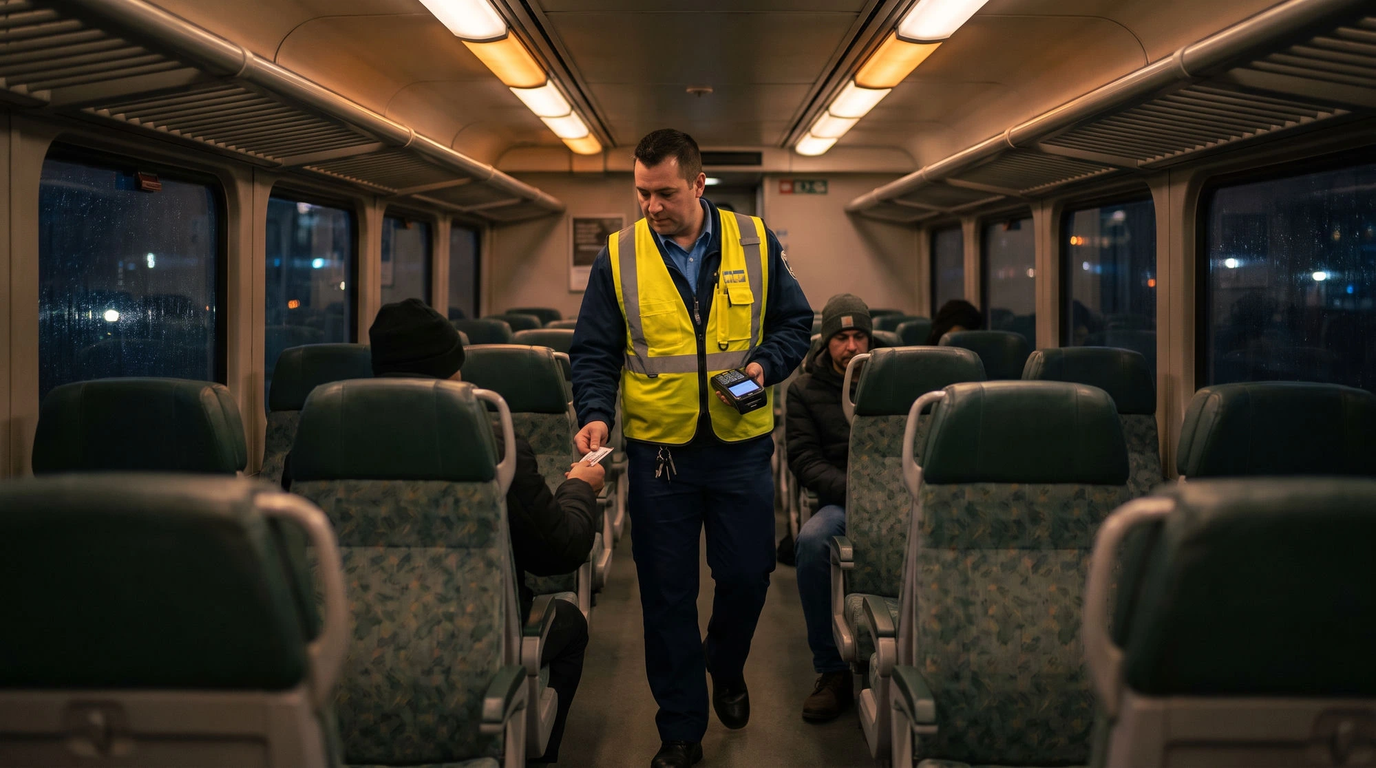
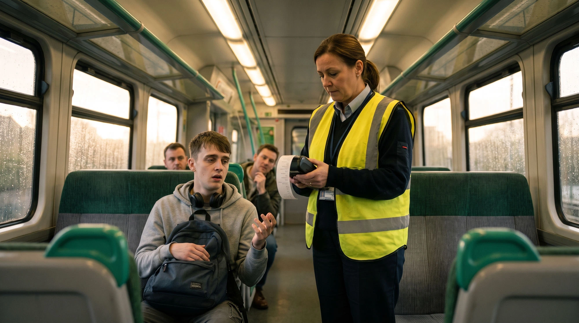
The moment the bet comes due: the ticket prints, and the rider does the arithmetic he should have done at the platform

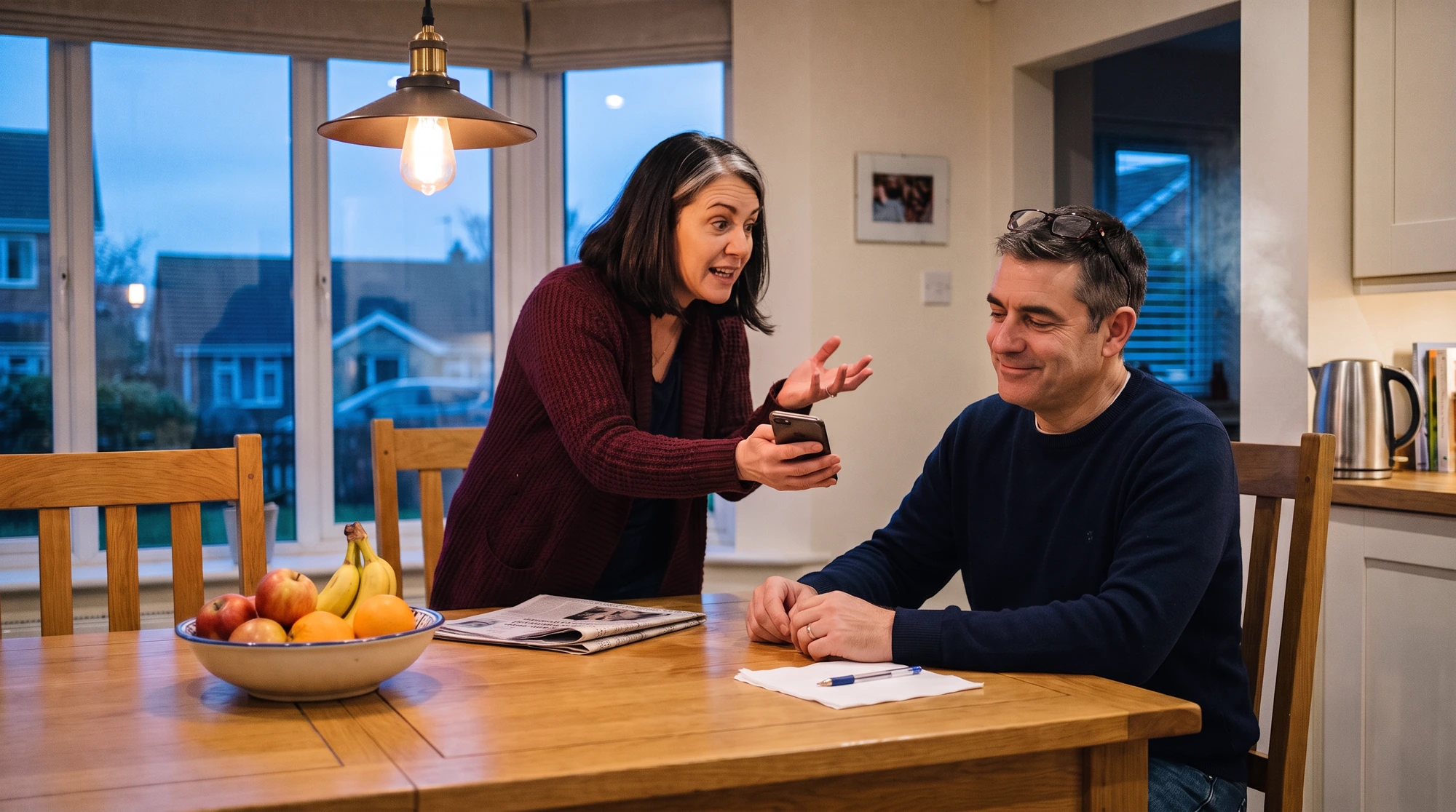
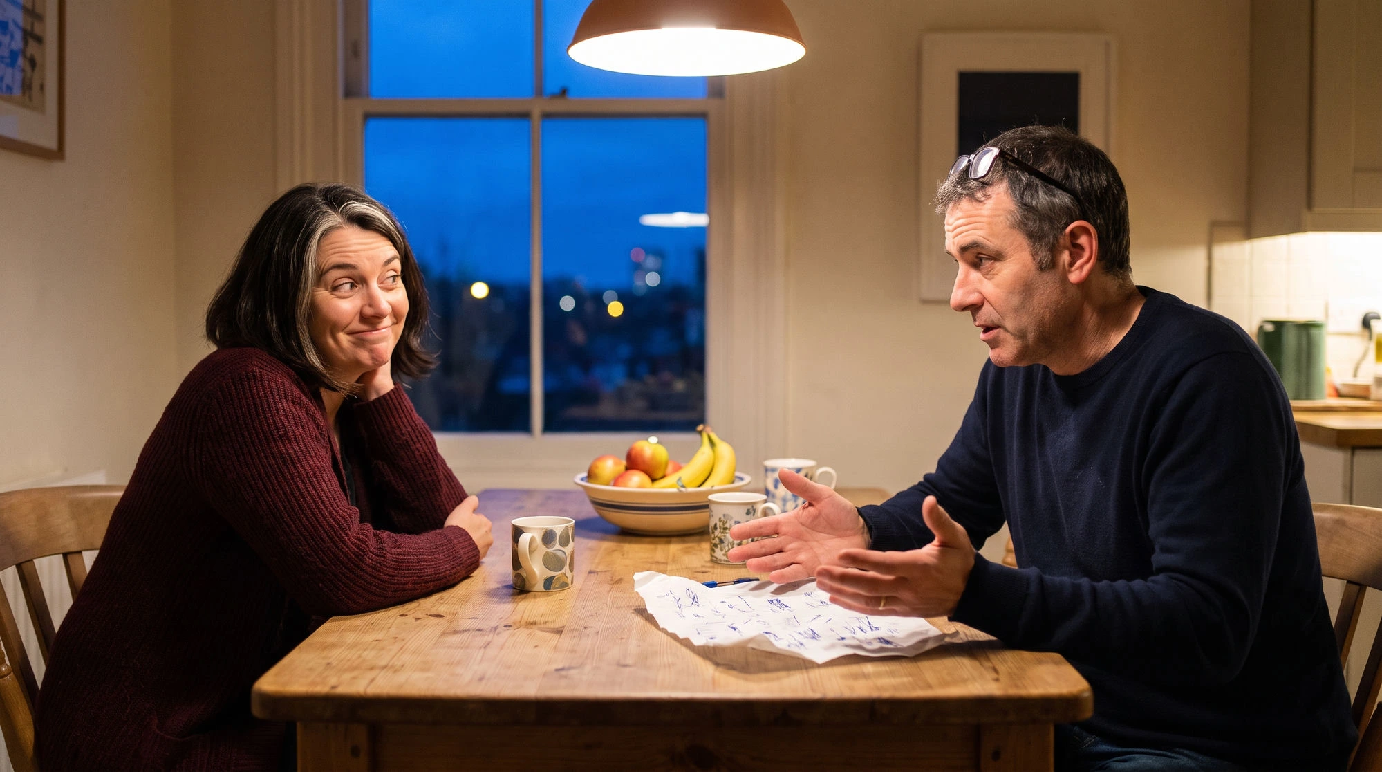
The kettle had just clicked off when my wife came into the kitchen, holding her phone at arm's length. Rain ticked against the window, and the headline on her screen was large enough for me to read before she said a word.

"Two hundred dollars," she said. "That is going to be the first fine for riding the train without paying. It starts September 8."

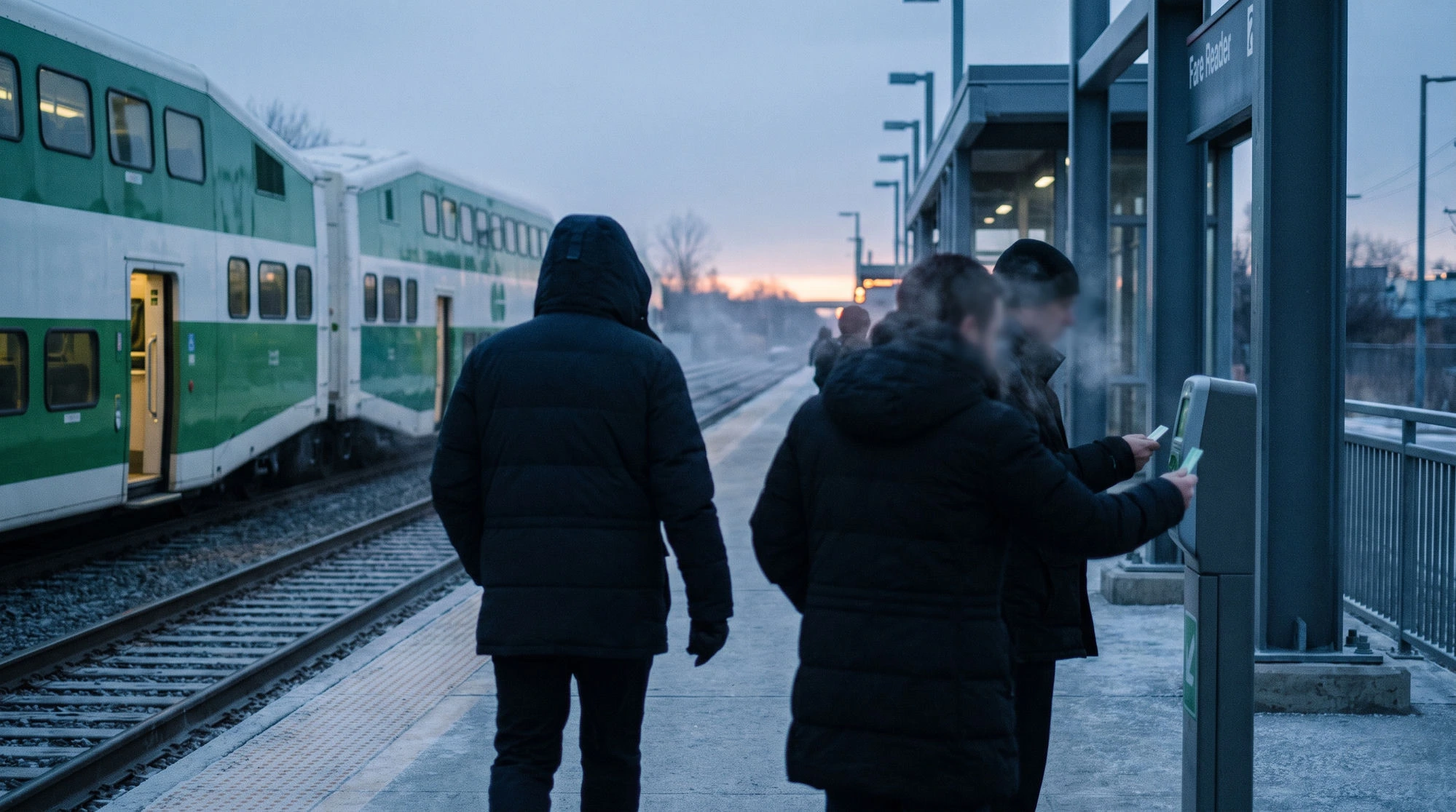
I smiled before I could stop myself. Not because two hundred dollars was funny, and not because I wanted anyone punished. I was thinking about the young man I often saw on the 7:42, the one who would slow down beside the card reader, glance at it, and keep walking.

My wife lowered the phone. "You are smiling at a two-hundred-dollar fine?"

"I am smiling because his decision changes on September 8, even if the trains, the inspectors, and the price of the ride all stay exactly the same."

"That sounds suspiciously like a defence of fare dodging."

"It is not a defence," I said. "It is a bet. The old rules made one kind of bet; the new rules make another. Give me that napkin."

Tuesday evening. The news arrives by phone, and for some reason he is smiling.

The bet nobody admits they are making

I drew two short branches. On one branch, you pay a ten-dollar fare and know exactly what the ride costs. On the other, you walk past the reader and pay nothing unless an inspector catches you. Ten dollars is only a round-number example, but it lets us see the wager clearly.

Let p be the probability of being caught on that ride. The expected cost of skipping is p multiplied by the fine. In this narrow money-only model, skipping has the lower expected cost whenever that amount is below the fare:

p × fine < fare

The interesting number is not the inspection rate itself. It is the point where the two branches become equal, the point where one more fraction of risk changes the answer:

p* = fare / fine

Under the old first-offence fine, the napkin said 10 / 35, or 28.6 percent. In other words, for this single-ride example, paying became cheaper on average only if the chance of being caught was greater than roughly two rides in seven.

That result does not make fare evasion honest, harmless, or wise. It also does not model the old penalties for repeat offences. It says something narrower, and more uncomfortable: when the immediate legal penalty is small, a person looking only at one ride and only at money can talk themselves into believing the gamble is rational.

My wife read the last line twice. "So the old fine was not large enough to frighten a calculator. What changes on September 8?"

Every rider who walks past the reader has made a bet. Most of them have never written it down.

What changes on September 8

I wrote September 8 across the top of the napkin and drew a line under it. The room had gone quiet except for the refrigerator and the rain.

The first change is the number in the headline. According to Metrolinx's announced schedule, a first offence rises from $35 to $200. In our ten-dollar example, p* becomes 10 / 200, or 5 percent. That is one chance in twenty. The same ordinary ride now sits on the other side of the calculation at a much lower inspection rate.

What the break-even inspection rate looks like Two rows of ride tiles. Under the old thirty-five dollar fine, paying only wins if more than two of every seven rides are inspected. Under the new two hundred dollar fine, paying wins if more than one of every twenty rides is inspected. Old fine, $35 paying only wins if more than 2 of every 7 rides are inspected (28.6%) New fine, $200 paying wins if more than 1 of every 20 rides is inspected (5%) Each tile is one ride. The red tiles are inspections at exactly the break-even rate. Any more than that, and paying is the cheaper bet on average.

The second change is the ladder. The penalties rise to $300 for a second offence, $400 for a third, and $500 for a fourth. A fifth brings a Provincial Offence Notice with a set fine established by the Chief Justice of the Ontario Court of Justice. A sixth or later offence brings a court summons and can mean a fine of up to $1,000 upon conviction. The fifth-offence amount is not stated in the announcement, so the cumulative total cannot honestly be called exactly $2,400. The first four fines plus a maximum sixth-offence fine already reach $2,400, and the fifth-offence set fine sits on top of that.

Every catch costs more than the last Bars show the announced penalties: two hundred, three hundred, four hundred, and five hundred dollars, then an unspecified set fine on the fifth offence and up to one thousand dollars upon conviction from the sixth. The known first four fines total fourteen hundred dollars; a maximum sixth-offence fine brings the known subtotal to twenty-four hundred dollars before the fifth-offence set fine is added. Every catch costs more than the last $0$500$1,000$1,500$2,000$2,500 a year of fares saved: 250 rides × $10 = $2,500 ? $200$500$900$1,400$2,400 + 5th fine 1st2nd3rd4th5th6th and after $200$300$400$500set finecourt, up to $1,000 Known total through the 4th: $1,400. A maximum 6th fine adds $1,000; the 5th-offence set fine is unstated.

This matters because a regular fare evader is not making the same one-ride gamble again and again. The downside becomes steeper after every catch. Imagine 250 ten-dollar commutes in a year. Never paying would preserve $2,500, but each offence takes a larger bite, and the later rungs add paperwork, court, time, and uncertainty that do not fit neatly into one dollar cell.

Catches in the yearFines so farAgainst $2,500 saved
1$200still $2,300 ahead
2$500$2,000 ahead
3$900$1,600 ahead
4$1,400$1,100 ahead
5$1,400 plus an unspecified set fineProvincial Offence Notice issued
6up to $2,400 plus the fifth-offence fineresult depends on that fine and the court outcome

Six catches in 250 rides is about 2.4 percent, or roughly one in forty-two. That is a useful warning line, not an exact expected-value threshold for the whole year. An exact model must account for the probability of every possible number of catches and the escalating penalty attached to each one. The napkin is showing how quickly the annual gamble can collapse, not pretending the staircase is a straight line.

My wife tapped the table beside the unknown fifth fine. "So even your scary total has a blank in it."

"Yes," I said. "A good model should show the blank, not hide it."

"And you still do not know the chance of being caught."

"No."

She pulled out the chair across from me and sat down. Until then I had been explaining a formula. Now we had reached the part that bothered both of us: how do you make a decision when the number deciding it is missing?

Two hundred, then three hundred, then four hundred. The ladder does not care that you only meant to do it once.

The number you do not need to know

I turned the napkin around so the five percent faced her. "This is the useful part," I said. "Not the fine, and not even the train. This line."

When a decision depends on a probability nobody can give you, the natural response is to hunt for it. You search reports, argue in forums, ask someone who knows someone inside the organization, and eventually discover that the number is uncertain, changing, confidential, or all three.

Threshold analysis starts from the opposite direction. Do not begin with, "What is p?" Begin with, "At what value of p would I change my choice?" For the simple first-offence ride, that threshold is exactly 5 percent under our assumptions. For the repeated-rider staircase, the roughly 2 percent figure is only a quick warning estimate; a full model is needed for the exact crossover.

The idea travels far beyond transit. A doctor may not know the exact probability of disease but can calculate the probability at which treatment becomes preferable to waiting. A product team may not know demand but can calculate the adoption rate needed to recover development cost. The threshold does not remove uncertainty. It gives uncertainty a boundary.

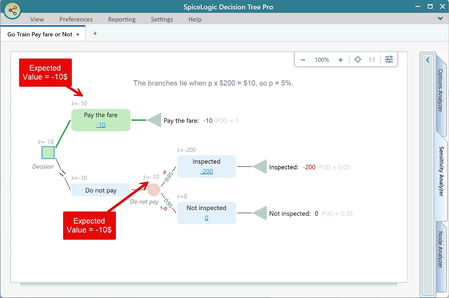
The fare decision as a decision tree A decision node with two branches. Pay the fare leads to a certain cost of ten dollars. Skip the fare leads to a chance node: inspected with probability p costs two hundred dollars, not inspected costs nothing. Board the train Pay the fare Skip the fare certain cost −$10 inspected, probability p not inspected, 1 − p −$200 $0 Expected cost of skipping = p × $200. It equals the fare when p = 10 / 200 = 5 percent.

The tree above contains the whole single-ride decision: one square for the choice, one circle for what happens next, and three monetary outcomes. The formula comes from those branches. You can calculate the crossing point without knowing the true value of p, provided you are honest about the assumptions behind the tree.

My wife touched the circled five. "So this is not your prediction of how often inspectors appear."

"Exactly. It is the border. I still may not know where reality is, but now I know the border it has to cross before my decision should change."

The crossing point. Left of it, skipping is cheaper on average. Right of it, paying is. You do not need to know where you stand on the line, only which side.

The question you can actually answer

My wife was not finished. "A border is useful only if you know which side you are standing on."

She was right. Your last twenty rides can be a rough reality check, but they are not a reliable estimate of the inspection probability. One check in twenty does not prove the rate is 5 percent, and no checks do not prove it is zero. Inspections can cluster by route, time, station, and enforcement campaign. Memory also edits the record.

Expected cost per ride against inspection probability Paying is a flat ten dollars. Skipping under the new two hundred dollar fine rises with probability and crosses ten dollars at five percent. Under the old thirty-five dollar fine it crosses at 28.6 percent. A separate marker at 2.4 percent illustrates six catches in 250 rides; it is not an exact annual expected-value threshold under escalating fines. 0%2%4%6%8%10%12% $0$5$10$15$20 Chance of an inspection on any one ride Expected cost of the ride skip, old $35 fine (crosses at 28.6%, off this chart) pay the fare: $10, every time skip, new $200 fine 2.4%: six catches in 250 rides, illustrative only 5%: the threshold one inspection in twenty rides skipping cheaper on average paying cheaper on average

The chart is the napkin drawn cleanly. The green line is the certain ten-dollar fare. The red line is the expected cost of skipping under a $200 fine. Their crossing is the 5 percent threshold. The dashed grey line shows the old $35 first-offence example, whose crossing sits far to the right at 28.6 percent.

What the chart gives you is not permission to replace data with a hunch. It gives you a disciplined question: does every plausible inspection rate lie on one side of the crossing, or does the answer change inside the range you consider believable? If the range straddles the threshold, the decision is sensitive and you need better evidence, a wider safety margin, or a rule that does not depend on expected value alone.

The only question that matters now: have you seen this man more than once in your last twenty rides?

Why I was smiling

"Then the people who walked past the reader were not necessarily stupid," my wife said.

"Not necessarily," I said. "But I would not call them correct either. Some may have done the arithmetic; some may simply have copied what others were doing. The narrow one-ride model only tells us that the old first-offence fine left room for a money-only argument. It says nothing about honesty, social cost, repeat penalties, or the kind of morning a court summons creates."

"And on September 8?"

"The new rules move the monetary threshold. Even if the inspection pattern stayed exactly the same, raising the first fine from $35 to $200 moves the simple break-even point from 28.6 percent to 5 percent. That is powerful, but it does not make inspectors irrelevant. A severe penalty deters only when people believe there is a real chance of being caught, that the fine will be collected, and that the rule will be enforced fairly. The policy changes one side of the wager; it does not solve all of human behaviour."

Where skipping stops being the cheaper bet A number line of inspection probability from zero to thirty percent. The single-ride break-even point moves from 28.6 percent under the old first-offence fine to 5 percent under the new one. The 2.4 percent marker represents six catches in 250 rides and is illustrative, not an exact expected-value threshold for the escalating ladder. How the first-offence fine moves the single-ride break-even point old $35 fine: single-ride break-even at 28.6% new $200 fine: single-ride break-even at 5% six catches in 250 rides: 2.4% (illustrative) 0%5%10%15%20%25%30% The 5% point is the exact single-ride threshold here. The 2.4% marker is only an annual warning line.

The province has estimated that fare evasion costs Metrolinx about $21 million a year. A larger fine makes the private monetary gamble less attractive, but the public problem is wider than one equation. Visibility of inspections, collection rates, accidental non-payment, ability to pay, and perceived fairness all affect what people actually do. Expected value can illuminate the incentive without pretending to settle the policy debate.

There was one last thing the average concealed. At the 5 percent threshold, paying and skipping have the same expected monetary cost, but they do not create the same life. Paying produces the same small loss every time. Skipping usually produces nothing, then occasionally produces $200, $300, $500, or a court date. A person minimizing the worst possible cost would pay. A person minimizing maximum regret would also pay. My wife looked at the napkin and said, "Averages never have to take a morning off work to go to court." That was the most important line written at the table, and it was not mine.

The same decision under three criteria A cost and regret grid. Paying costs ten dollars whether or not you are inspected, with a regret of ten dollars when you are not. Skipping costs two hundred dollars if inspected, with a regret of one hundred ninety dollars, and nothing otherwise. Minimizing worst-case cost and minimizing maximum regret both favour paying at any probability. The same decision under three criteria Inspected (p) Not inspected (1 − p) Pay the fare Skip the fare cost $10 cost $10 cost $200 cost $0 regret $0: you did the best thing regret $10: you could have ridden free regret $190: you could have paid $10 regret $0: you did the best thing Worst case pay: $10, skip: $200 minimax cost picks paying, at any p Biggest regret pay: $10, skip: $190 minimax regret picks paying, at any p Expected value needs p and flips at 5%. Worst case and regret need no p at all, and both pick paying whatever the inspectors are doing.
She got it before I finished the sentence. Most people do.

The lesson you take off the train

By then the tea was cold. The train had almost disappeared from the conversation, which is how I knew the example had done its job. Two ideas remained.

The first is expected value. Multiply each outcome by its probability, add the results, and you get the long-run average for repeating that choice under the model. It is useful when comparing certainty with risk, but it is not a moral verdict and it is not a promise about what will happen on your next ride. This is an expected value real-life example precisely because the arithmetic is simple and the human decision is not.

The second idea is threshold analysis. When an uncertain probability controls the answer, calculate the value at which the preferred option flips before spending days chasing a perfect estimate. Then compare that threshold with the evidence and with a realistic range of uncertainty. A doctor, an investor, a product manager, and a commuter can all use the same move.

A threshold turns "I do not know the probability" into a sharper question: "Would any believable value change my choice?" If the answer is no, the decision is robust. If the answer is yes, you have learned exactly which uncertainty deserves attention.

The arithmetic does not know Toronto. Replace the ten-dollar fare and the $200 fine with the numbers from your own city, and the single-ride threshold is still p* = fare / fine. Just remember what the napkin taught us: repeated penalties, missing amounts, imperfect data, and human risk preferences belong in the story too.

The sixth rung of the ladder is not a fine. It is a morning here.

Doing this with a real decision tree

A napkin is enough for one choice, one uncertain event, and two clean outcomes. Real decisions rarely stay that polite. They branch, repeat, carry several costs at once, and hide the probability you care about three levels deep. That is where a proper decision tree earns its place.

In Decision Tree Pro, you can build the same basic structure shown above, then expand it without losing the logic: a decision node, chance nodes, probabilities, and payoffs. The Sensitivity Analyzer varies an uncertain input across a range and draws the competing expected values, so the crossing point becomes visible instead of buried in algebra. On a larger model, the sensitivity index helps separate inputs that can change the decision from inputs that merely look important. You can also compare expected value with a worst-case rule or minimax regret rather than forcing every decision into one criterion.

The sensitivity analysis guide demonstrates the same logic with a job-offer decision. When observations later become available, the Bayesian inference tools can update the probability while preserving the uncertainty around a small sample. A dozen rides and one inspection do not create certainty; they create evidence, which is a different and more honest thing.

The next morning, the platform was still wet. The young man from the 7:42 slowed beside the card reader, just as he always did. I looked away before he chose. My wife tapped her own card, and the reader gave its ordinary green chirp. "Five percent is not very much," she said. The napkin was still folded in my coat pocket. The mathematics had taken three lines. The decision, as usual, still belonged to a person.

Related product Decision Tree Software
Last modified Sep 4, 2026

© All content, photographs, graphs and images in this article are copyright protected by SpiceLogic Inc. and may not, without prior written authorization, in whole or in part, be copied, altered, reproduced or published without exclusive permission of its owner. Unauthorized use is prohibited.